Just here for the pictures? Jump straight to the Results.

Problem Statement

I’ve recently started implementing an atmosphere model for my renderer and quickly realized something frustrating: no matter how much I tweak the Rayleigh, Mie, and ozone coefficients, I can’t get a render that looks right across all conditions.

I can tune the parameters to produce beautiful, blue skies when the sun elevation is high but the moment the sun is low on the horizon I can’t get a decent rendering. The image becomes too red with high absorption or completely lacks the decent purples that show in twilight conditions without enough ozone as one can see in the below photograph.

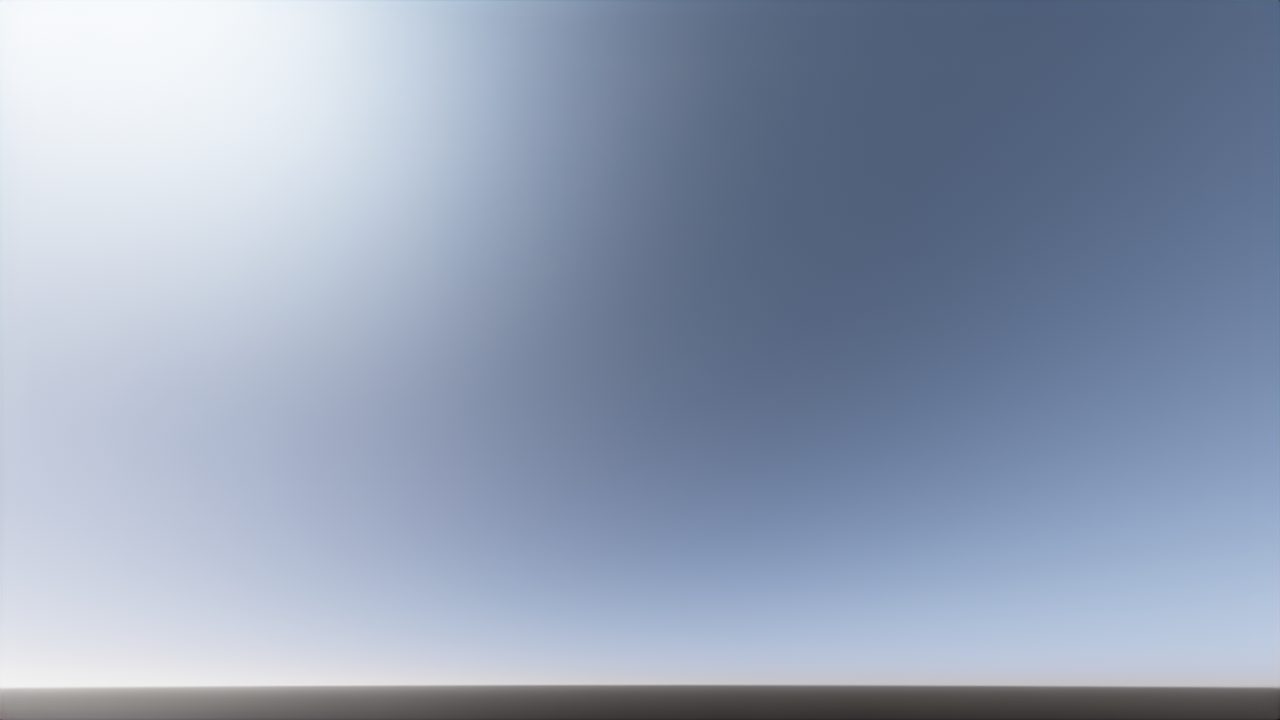
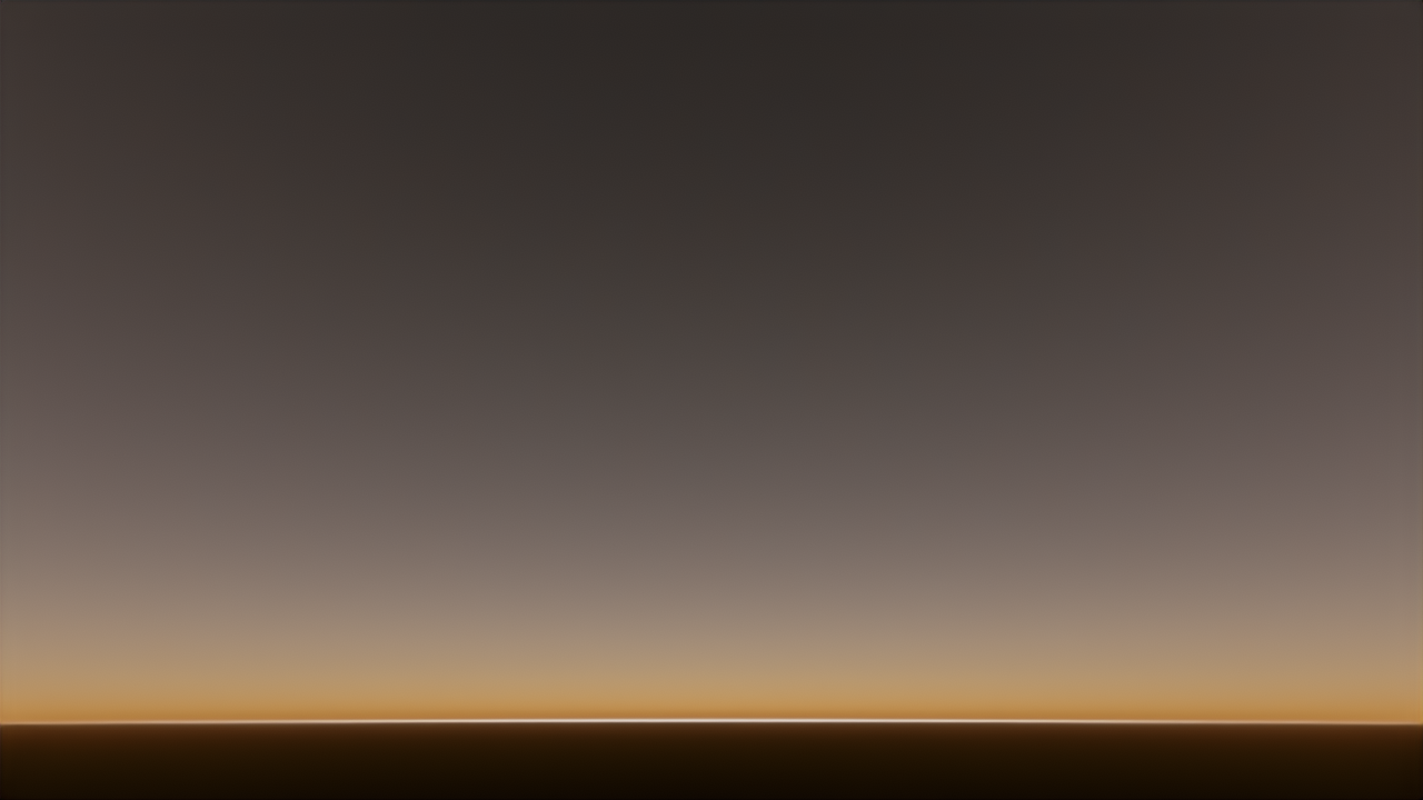
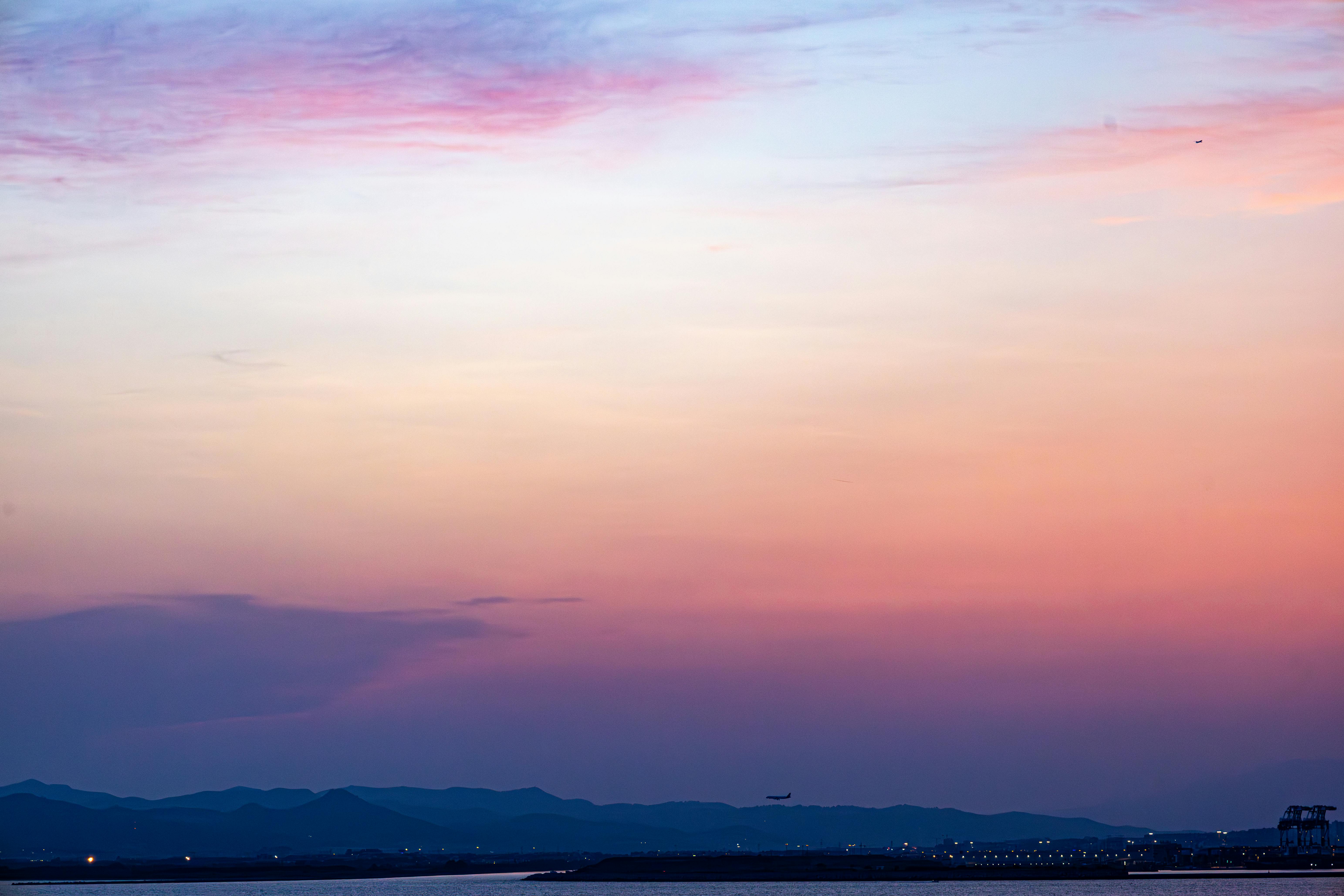
image credit @ Regan Dsouza

The deeper I dug, the clearer the root cause became: RGB rendering simply doesn’t have enough spectral resolution to model atmospheric scattering faithfully. Rayleigh scattering is a strongly wavelength-dependent phenomenon — its cross-section scales as λ⁻⁴. When you collapse the full solar spectrum down to three broad RGB channels, you’re throwing away exactly the information that makes the sky look like the sky. You can fudge coefficients to look plausible in one lighting condition, but there’s no single set of RGB values that generalizes across sun angles, altitudes, and times of day.

Motivation

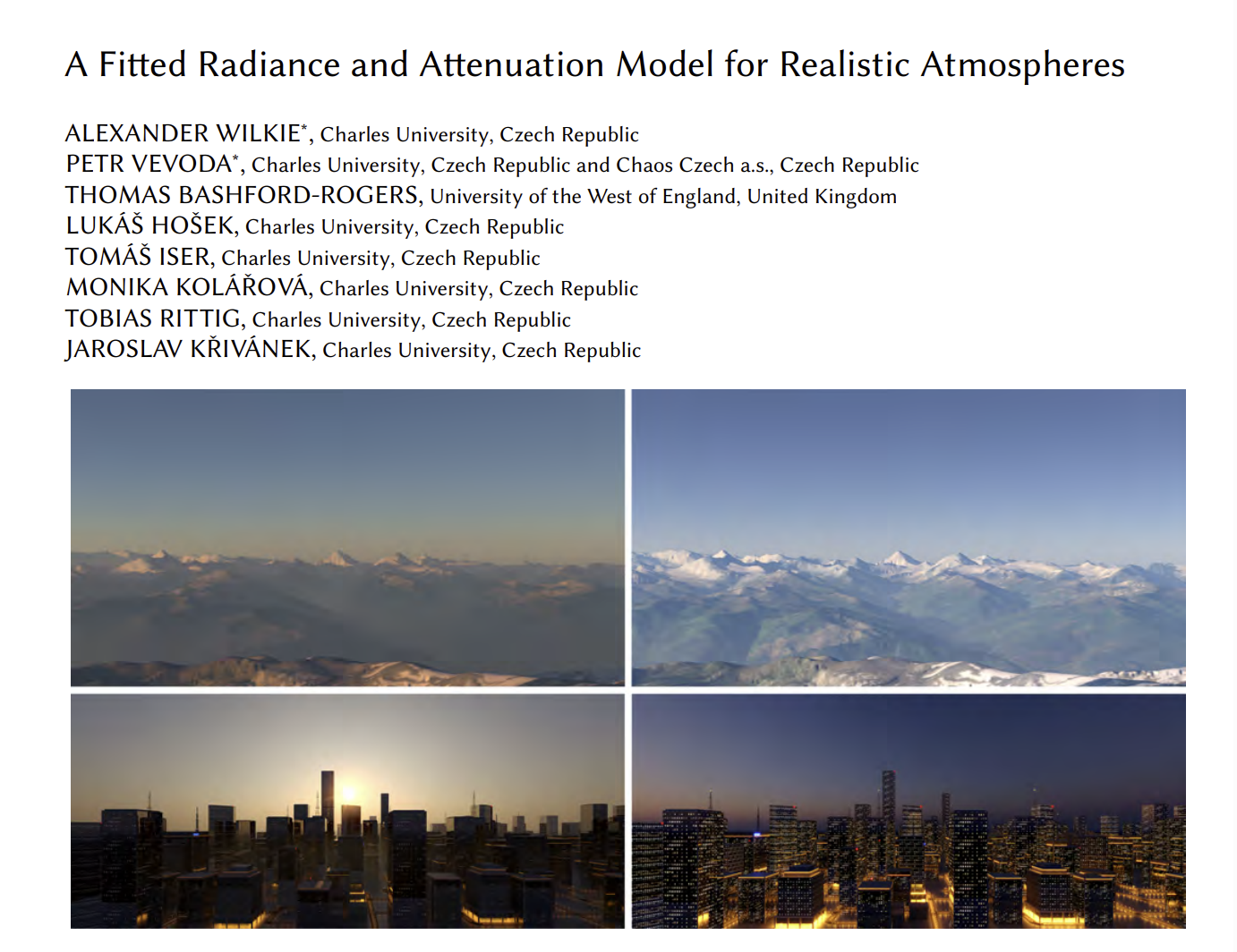
While digging into the problem, I came back to a 2021 paper I had read: A Fitted Radiance and Attenuation Model for Realistic Atmospheres by Wilkie et al. In this paper the authors mention that they’ve built a brute-force simulation engine called atmos_sim alongside their fitted model — a path tracer that integrates atmospheric scattering directly from real-world physical data, with no precomputation or fitted approximations. It’s the ground truth their fitted model is trained against.

That gave me an idea. Instead of continuing to fiddle with RGB coefficients in my main renderer, I could implement my own version of atmos_sim. This would serve two purposes:

First, it would let me stress-test the delta tracking and transmittance computation already in my renderer. These are the same routines that power my current atmosphere model, and I’ve never had a clean reference to validate them against. A standalone brute-force path tracer, built on the same physical data, would tell me definitively whether the math is right or whether the bugs I’m chasing are somewhere deeper.

Second, it would give me a spectral ground truth I can diff against my main render engine. If I can render the same scene in both and compare, I’ll be able to see exactly where and how the RGB approximation breaks down — and make more informed decisions about where to invest effort next.

So that’s the goal: a self-contained, brute-force, spectral atmospheric path tracer built on real physical data, no precomputed tables, no fitted models.

Getting Data

Like Wilkie et al., I sourced the physical data from libRadtran — a well-established library for radiative transfer calculations that ships with a comprehensive set of measured atmospheric data. Despite covering everything needed for a full spectral simulation — density profiles, scattering coefficients, ozone absorption cross-sections, aerosol properties, and solar irradiance — the total data footprint came out to well under a megabyte.

Density Profiles

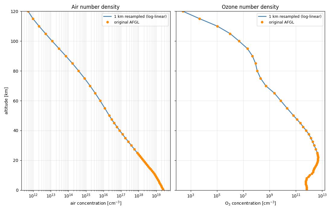
Atmospheric density data was extracted from libRadtran using the US Standard Atmosphere profile — a widely used reference model that tabulates air and ozone concentration as a function of altitude.

The raw data isn’t linear in altitude, so a direct linear interpolation between sample points would introduce noticeable error. Instead, I re-fit the data using log-linear interpolation, which respects the exponential nature of atmospheric falloff much more faithfully. The result is a compact, accurate representation of both air and ozone number density as a function of altitude in kilometers.

Rayleigh Scattering Coefficients

Rather than pulling Rayleigh cross-sections from a table, I computed them analytically from first principles using the formulation from Bodhaine et al. (1999), which is the same source used by Wilkie et al.

The cross-section for a given wavelength is derived in three steps. First, the real refractive index of dry air is computed from the wavelength using the Peck & Reeder dispersion formula. Second, a King correction factor is applied to account for the fact that N₂ and O₂ molecules are not perfectly spherical — they scatter slightly anisotropically, which boosts the effective cross-section by a small but wavelength-dependent amount. Third, the two are combined into the standard Rayleigh cross-section formula, which carries the characteristic λ⁻⁴ dependence responsible for the blue sky.

The output is a table of scattering cross-sections in cm²/molecule, sampled from 320 nm to 760 nm in 1 nm steps — covering the full range from near-UV through the visible spectrum.

Ozone Absorption

Ozone absorption cross-sections were taken from the Serdyuchenko & Gorshelev (2013) dataset — specifically the July 2013 version, which has a Fast Fourier Transform filter applied to the raw data in the 213–317 nm region to reduce measurement noise. This is one of the standard reference datasets for ozone spectroscopy and is included in libRadtran directly.

From this dataset I exported only the 223 K temperature profile, sampled from 320 nm to 760 nm in 1 nm steps. 223 K corresponds roughly to the tropopause region where ozone concentration peaks, making it a reasonable single-temperature approximation for a first implementation.

It’s worth noting that libRadtran also ships per-altitude temperature profiles, which would allow computing temperature-dependent ozone absorption at each atmospheric layer rather than using a fixed 223 K value. That would be a more physically accurate approach, and something worth revisiting later.

Aerosol Particles

Aerosol data was the most complex part of the extraction pipeline. The atmosphere isn’t made of just air and ozone — it also contains suspended particulate matter, and these particles scatter and absorb light in ways that vary strongly with both wavelength and altitude.

I used three aerosol components from libRadtran’s OPAC (Optical Properties of Aerosols and Clouds) database, which ships pre-computed Mie scattering tables for common particle types:

• WASO (Water-Soluble) — hygroscopic particles like sulfates and sea salt, whose optical properties vary with relative humidity
• INSO (Insoluble) — mineral dust and coarse soil particles
• Soot — black carbon from combustion, strongly absorbing across all wavelengths

For each particle type, the data includes extinction coefficients, single-scattering albedo (the ratio of scattering to total extinction), and an asymmetry parameter derived from the phase function moments. The script then loads a standard continental_average profile that gives the mass concentration (g/m³) of each component as a function of altitude.

For each wavelength from 320 to 760 nm, all three components are combined into a single set of bulk aerosol properties at each altitude layer — total extinction, effective single-scattering albedo, and effective asymmetry — by weighting each component’s optical properties by its mass concentration. WASO properties are evaluated at 50% relative humidity. The combined values represent what a renderer needs: a single participating medium with one extinction value, one scattering albedo, and one phase function parameter per altitude per wavelength.

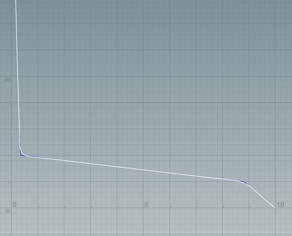
The raw profile data is coarse, with sparse altitude samples and a particularly sharp, unresolved feature around 1 km where aerosol loading changes quickly. To deal with this, I imported the per-wavelength CSV exports into Houdini, converted the altitude profiles to curves, applied curve smoothing, and then re-sampled them at a fixed uniform interval. This gave a clean, dense altitude representation that interpolates well at runtime.

An alternative approach would be to keep the three components separate — exporting their individual optical properties and concentration tables — and combine them inside the renderer. I chose to pre-combine because the resulting data stayed small enough to be manageable, but the per-component approach would allow things like per-species concentration tweaking without re-exporting everything.

Implementation Details

The renderer is a CUDA kernel running on an RTX 3090. Each pixel gets one thread, and the full Monte Carlo loop — spectral sampling, delta tracking, shadow rays, and multi-bounce integration — runs entirely on-device. All atmospheric data is uploaded to device memory once at startup.

The camera supports two equidistant fisheye modes: zenith-up (image center = zenith, edge = horizon) and horizon (camera axis pointing forward for a full spherical panorama).

The atmosphere is a concentric shell geometry with analytical ray–sphere intersection. The column is split into a lower segment (0–15 km) and an upper segment to keep delta-tracking majorants tight, since aerosol and dense Rayleigh scattering are concentrated near the surface.

Scattering events are found via delta tracking using a single hero wavelength per sample to drive free-path sampling. The hero wavelength cycles through the spectral bins across the pixel’s sample budget. At each step a candidate position is accepted as a real collision or rejected as a null collision, with ratio-tracked transmittance updated accordingly. Rayleigh scattering uses the analytic phase function; Mie scattering uses Henyey–Greenstein with the asymmetry parameter g from the pre-combined OPAC data.

Shadow transmittance is computed spectrally using the biased version of estimator from An Unbiased Ray-Marching Transmittance Estimator (Novák et al., 2021), which adapts its step count to the local optical depth rather than marching a fixed number of steps. Multiple scattering is handled by extending the bounce loop — after each scatter event a new direction is drawn from the phase function and the path continues, with a per-wavelength throughput array carrying the spectral weights forward across bounces.

Each wavelength’s contribution is accumulated into CIE XYZ via the color matching functions and converted to linear RGB at the end.

Results

All images in this section are rendered at 1024×1024 resolution and -otherwise stated- denoised. The metadata states the number of volumetric bounces, number of channels evaluated, number of samples and the cuda kernel render time in milliseconds.

Multiple Scattering

Of all the variables in this renderer, the number of scattering bounces has the single biggest impact on whether the sky looks physically real. A single-bounce sky is a fundamentally different — and wrong — thing: it misses all the light that has scattered more than once before reaching the camera, which in practice means the horizon is too dark and the characteristic colour gradients that make a sky feel alive simply aren’t there.

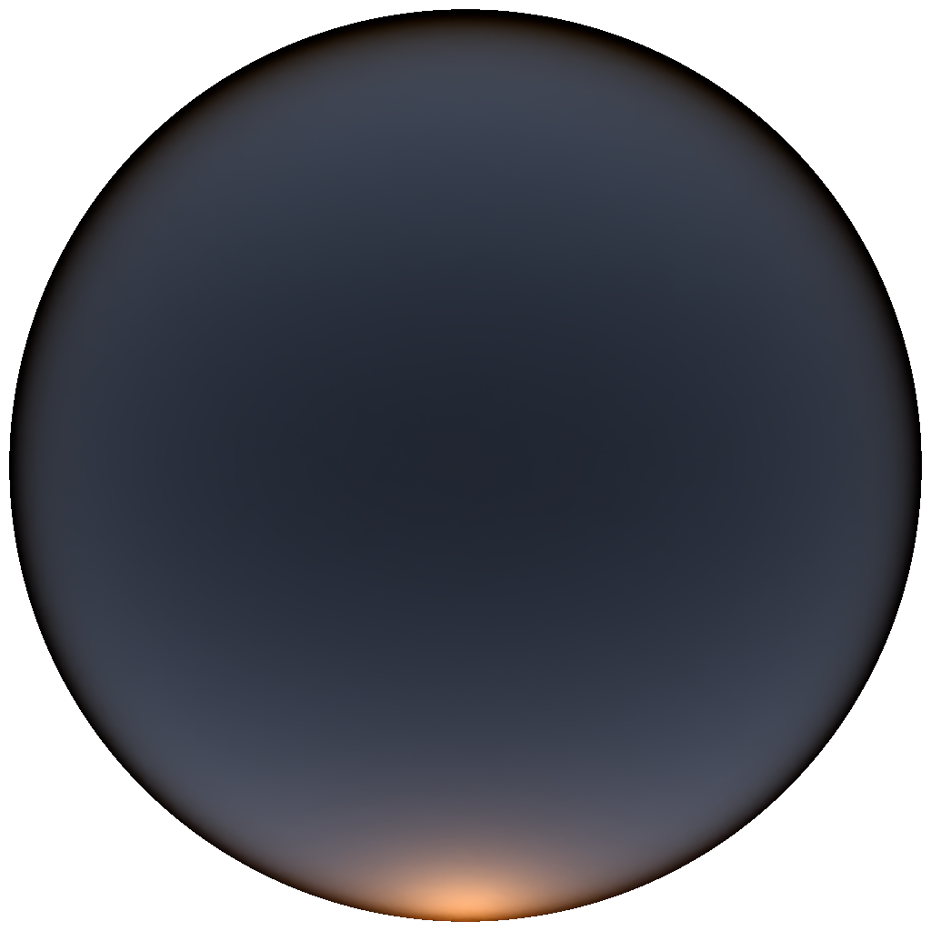
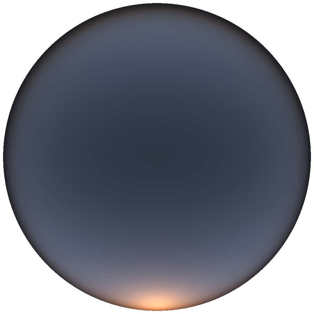
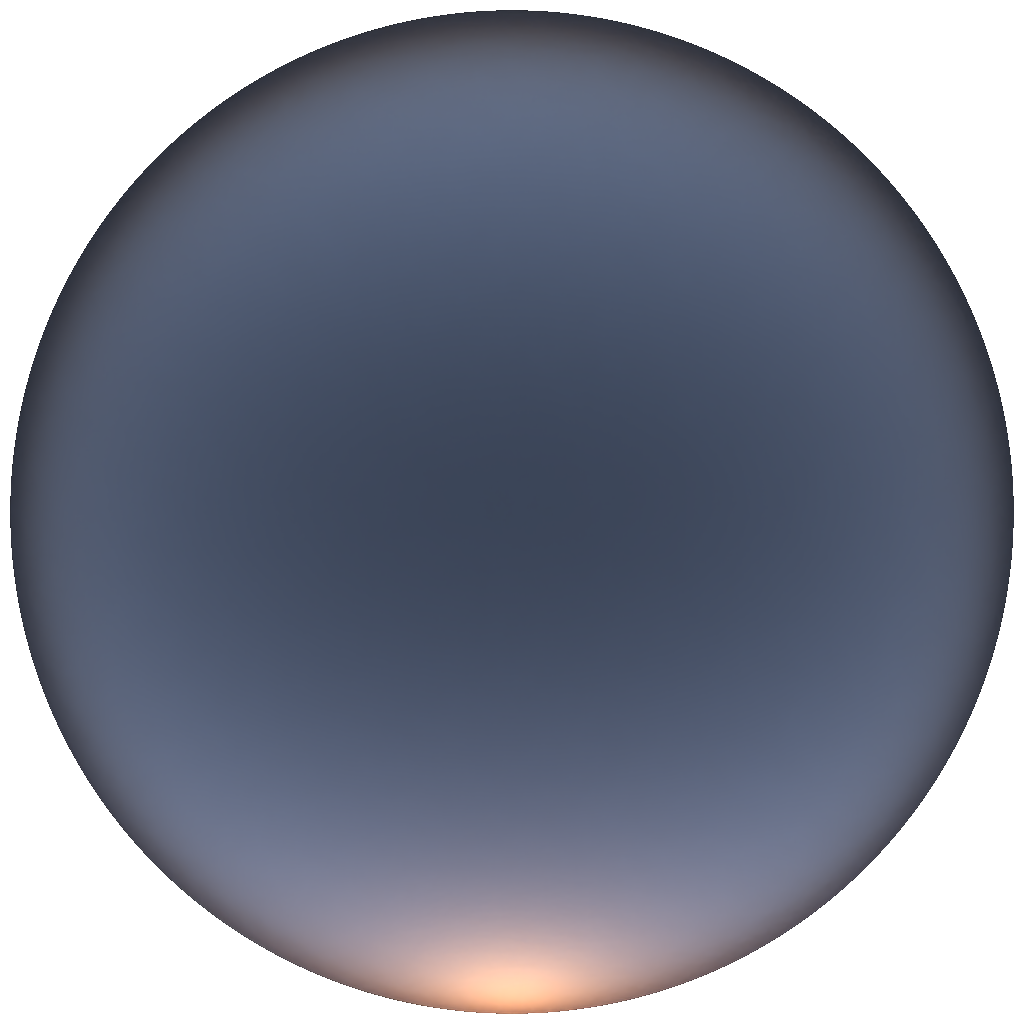
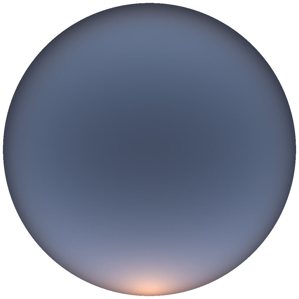
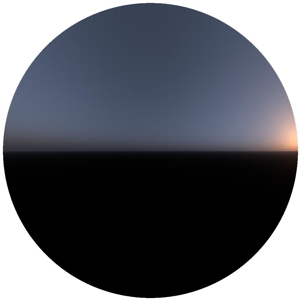
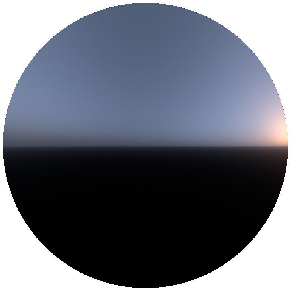
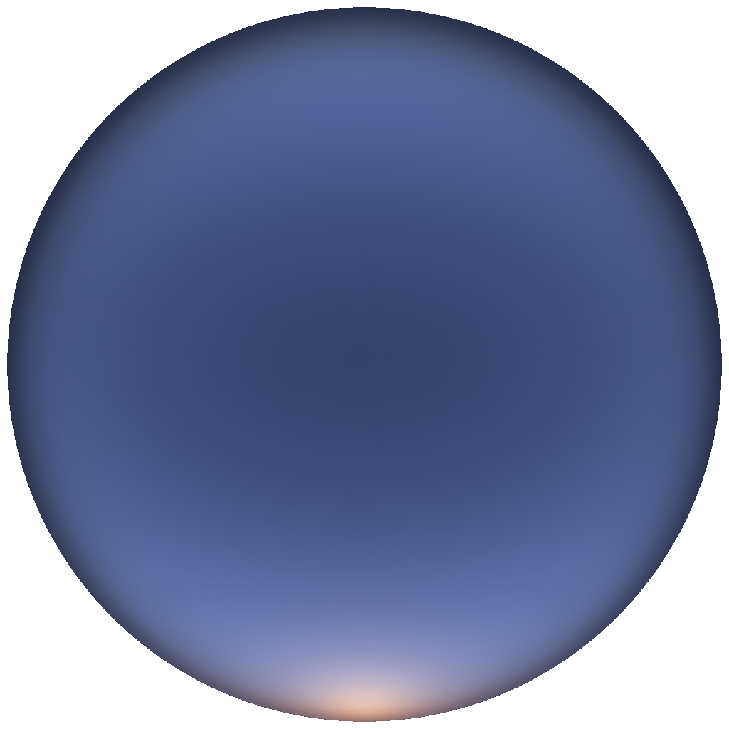
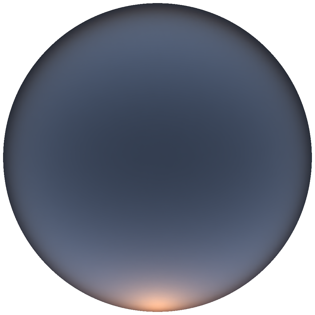
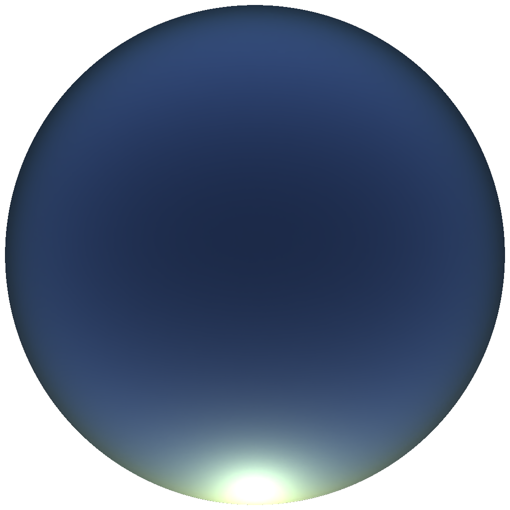
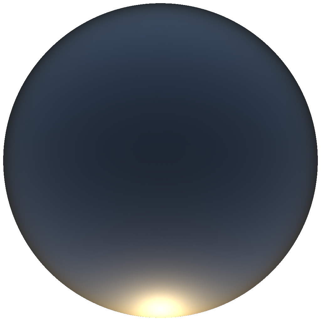
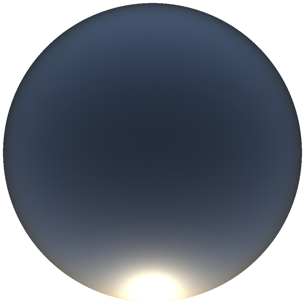
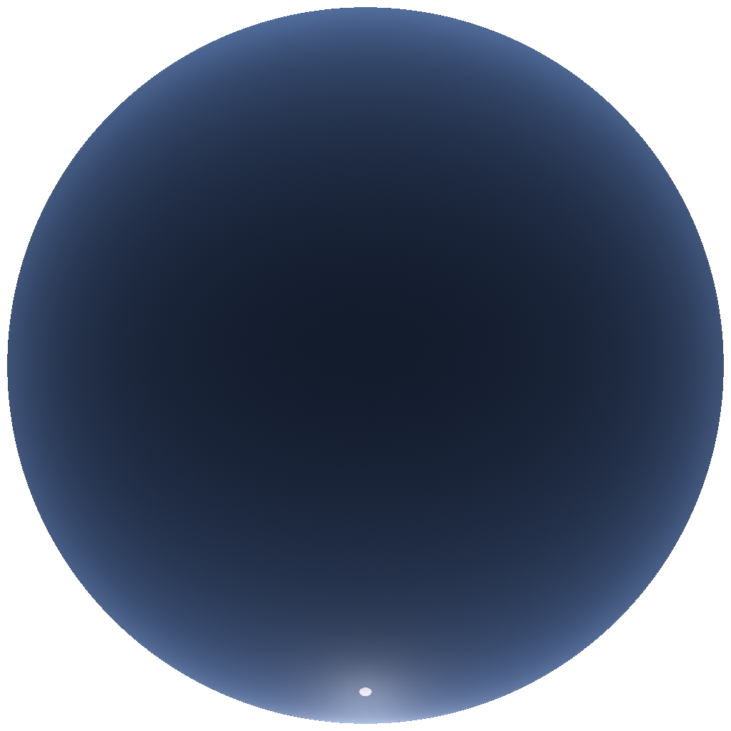
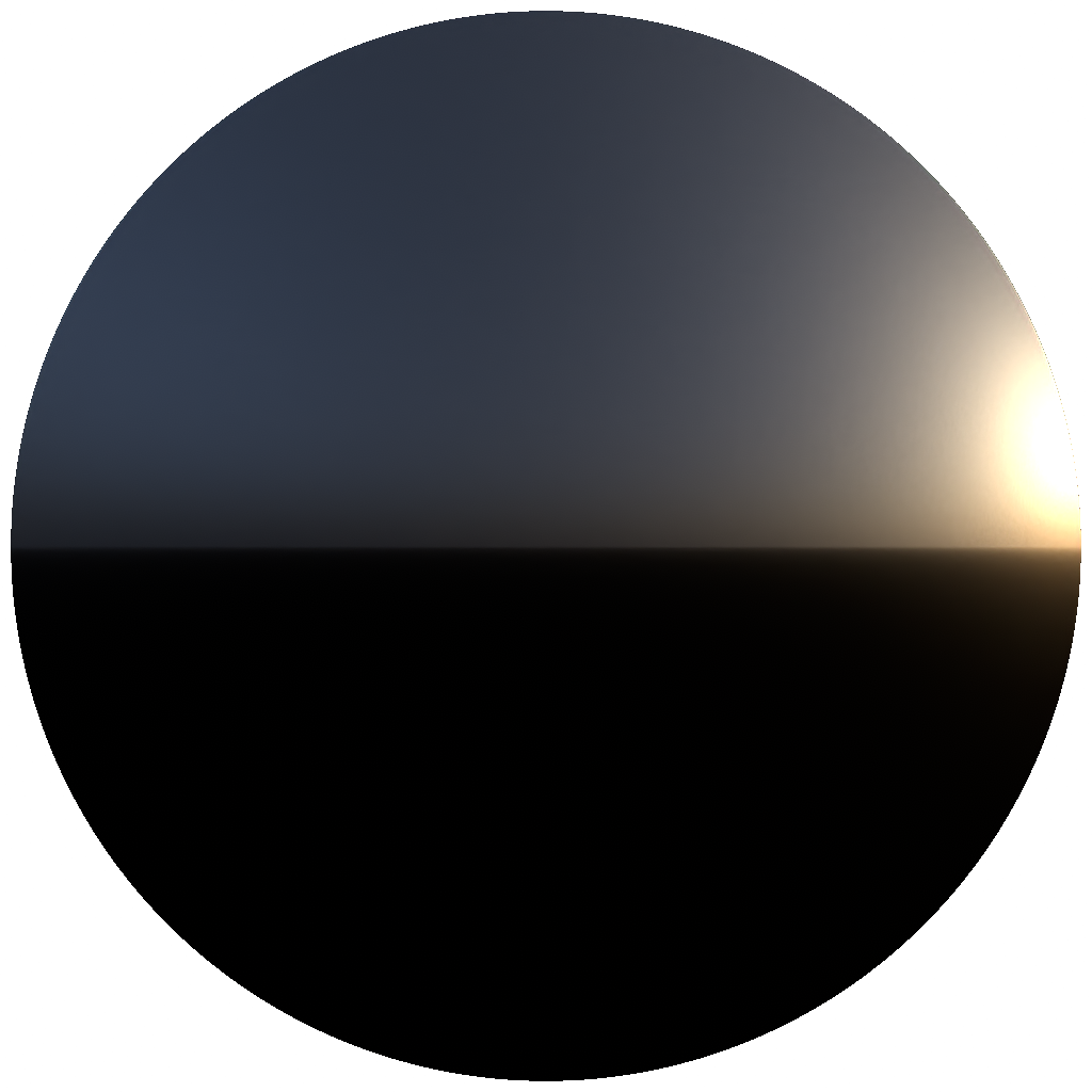
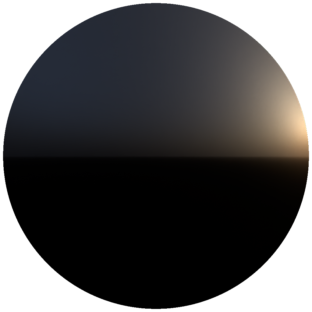
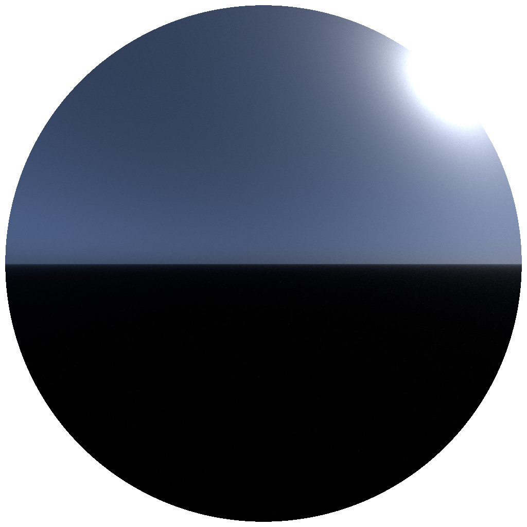
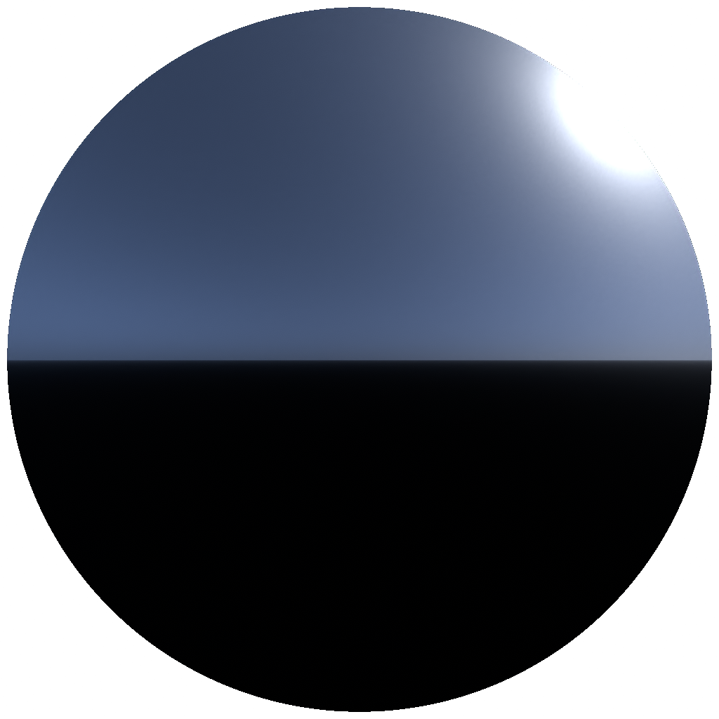
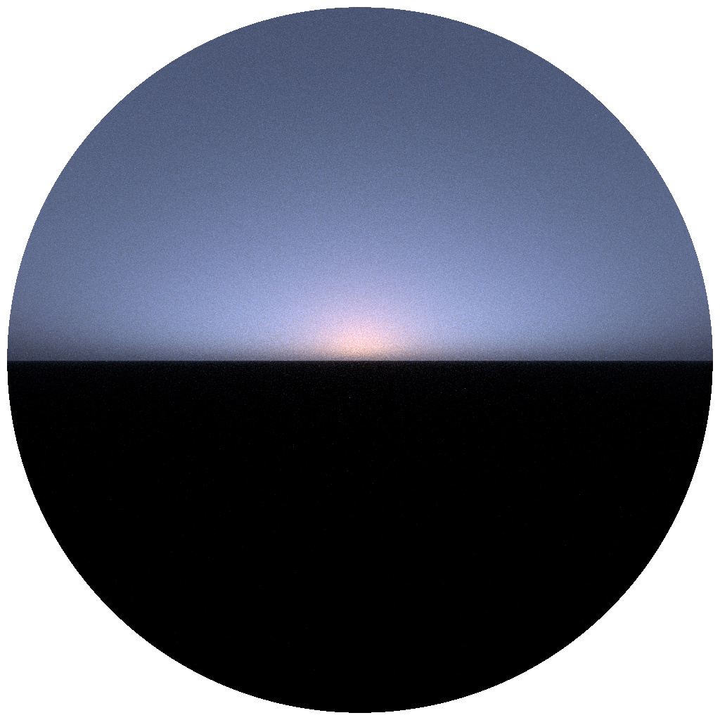
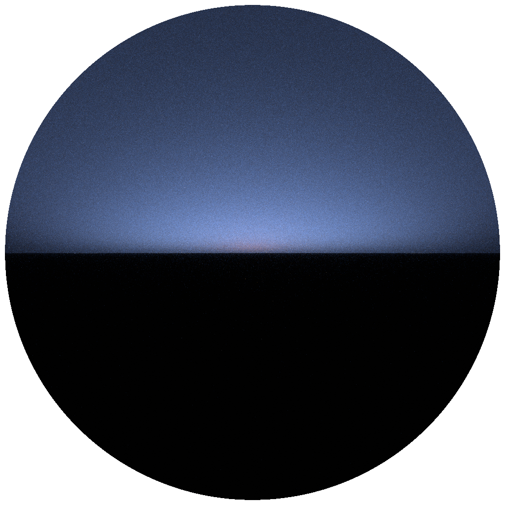
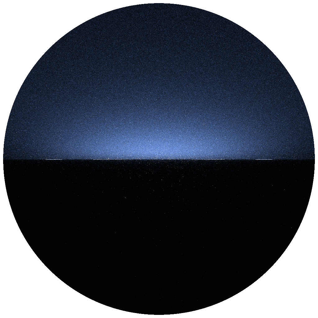
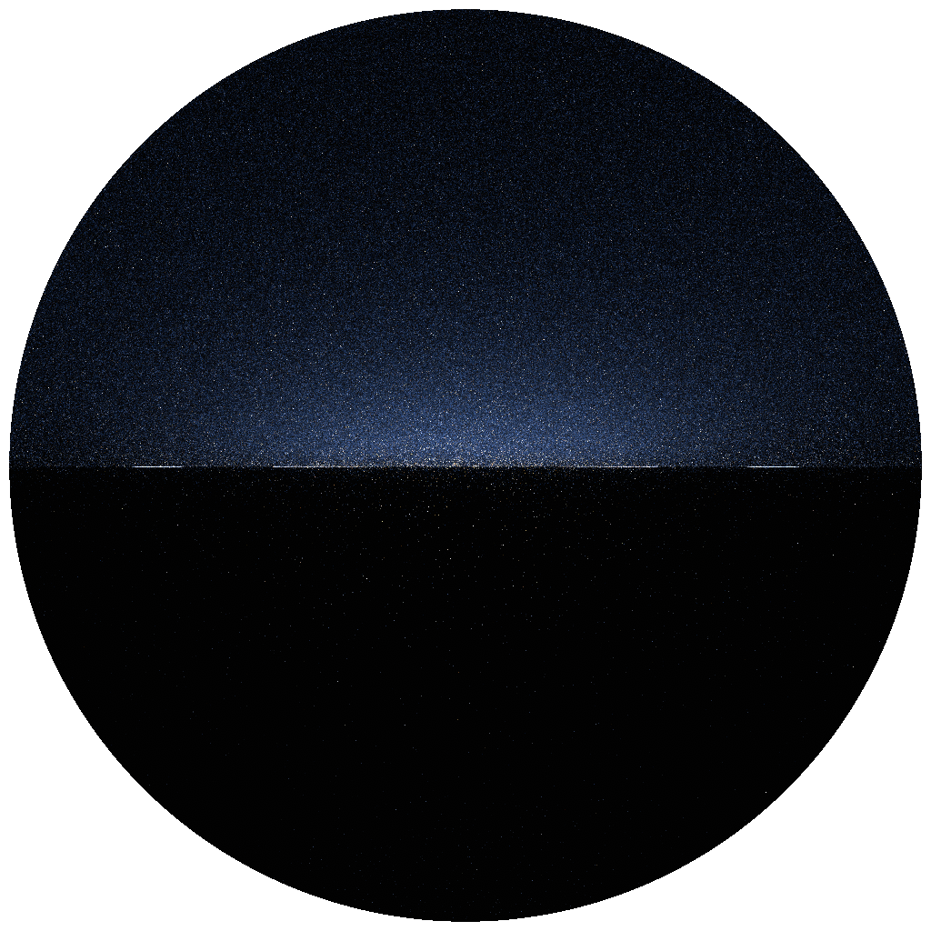
The images below show the sky with 1, 2, 4, and 8 bounce depths, rendered with the sun at the horizon where multiple scattering has the most visible impact. The zenith-up fisheye is shown on the top row; the horizon panorama on the bottom.

Zenith-up camera

Bounces: 1 · 40 λ · 1024 spp · 4689.39 ms	Bounces: 2 · 40 λ · 1024 spp · 9194.84 ms	Bounces: 4 · 40 λ · 1024 spp · 18083.7 ms	Bounces: 8 · 40 λ · 1024 spp · 35835.2 ms

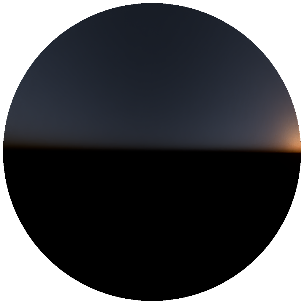
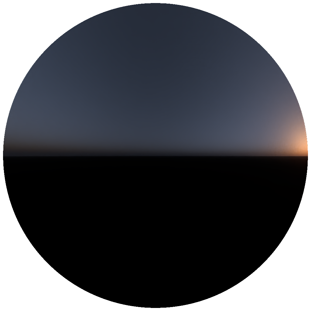
Horizon camera

Bounces: 1 · 40 λ · 1024 spp · 2929.08 ms	Bounces: 2 · 40 λ · 1024 spp · 5800.38 ms	Bounces: 4 · 40 λ · 1024 spp · 11664.9 ms	Bounces: 8 · 40 λ · 1024 spp · 23957 ms

With only a single bounce the horizon band is dark and the sky looks optically thin. From two bounces onwards the characteristic purple-violet hue builds up at the anti-solar horizon — the very effect that was impossible to reproduce in the RGB renderer.

Spectral Channels: 3 vs 40

The most direct demonstration of why the brute-force approach is worth it. The left column uses only 3 spectral channels (RGB) at 440nm, 540nm and 640nm; the right uses 40 channels spanning 320–760 nm. Both rows use the same number of bounces and sample count — the only variable is spectral resolution.

Sun at horizon (0° elevation)

Wavelengths: 3 · Bounces: 4 · 1024 spp · 5371.54 ms	Wavelengths: 40 · Bounces: 4 · 1024 spp · 67510.3 ms

At low sun angles the image looks like a plausible blue sky. At 5 degrees however the 3-channel version blows out into an unconvincing green. Note that this is still using per-wavelength volumetric scattering — in a pure RGB renderer, σ_t would be averaged across channels before the scatter point is selected, which would compound the error further.

High sun elevation (5° elevation)

Wavelengths: 3 · Bounces: 4 · 1024 spp · 5492.89 ms	Wavelengths: 40 · Bounces: 4 · 1024 spp · 67230.1 ms

Camera Altitude

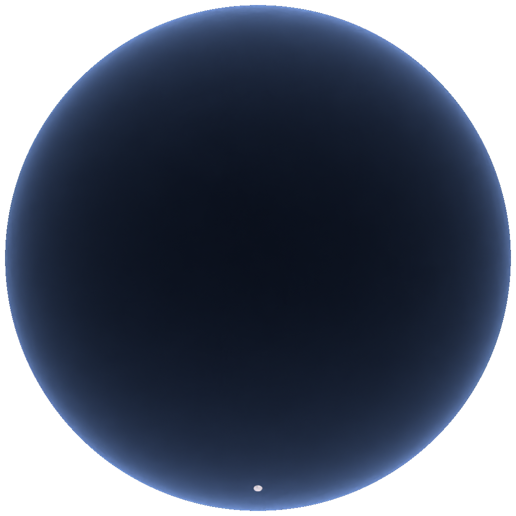
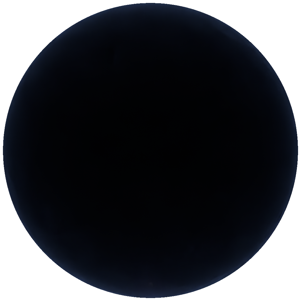
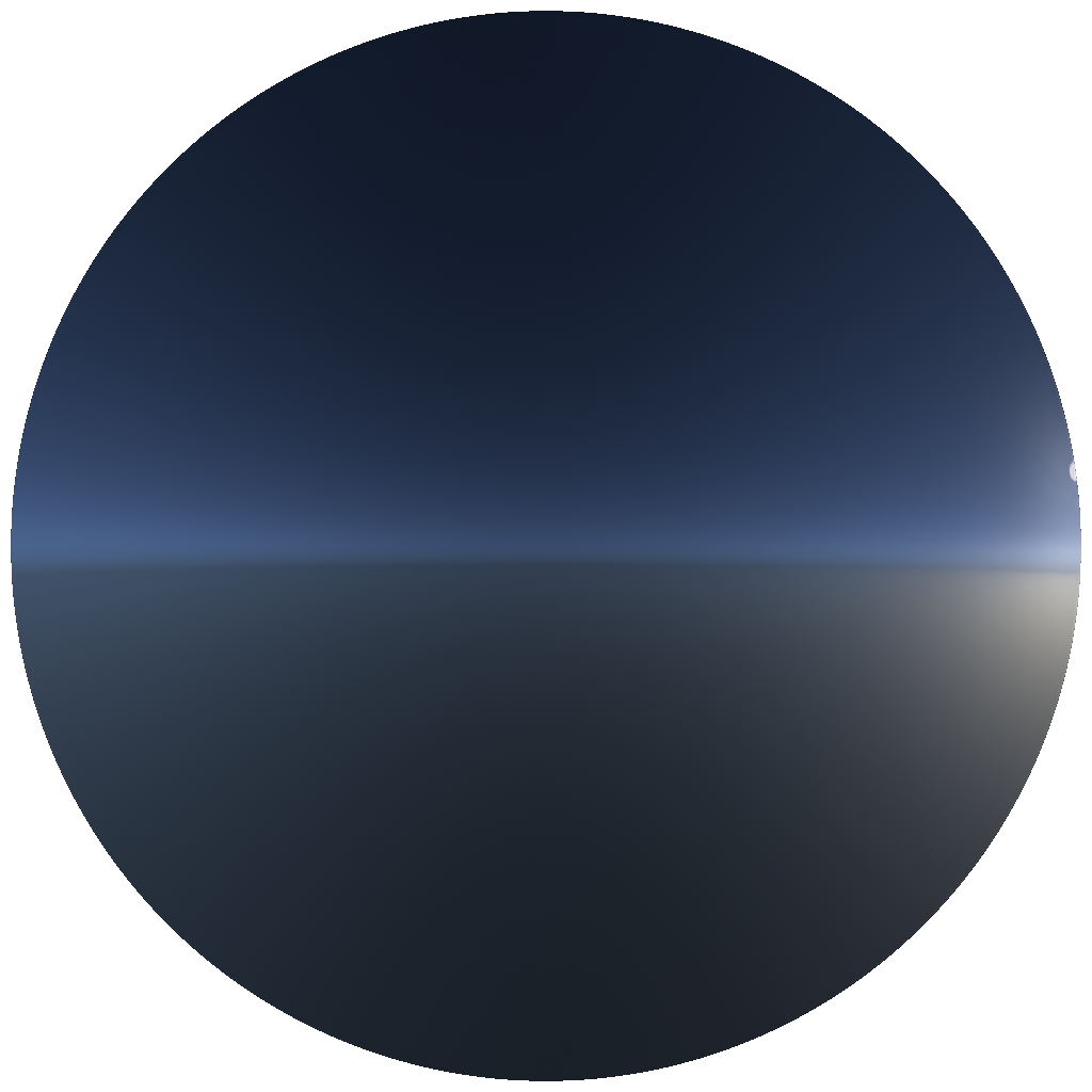
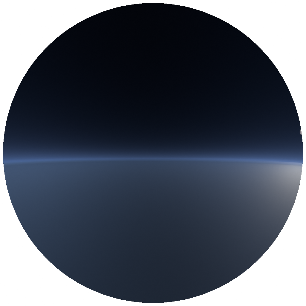
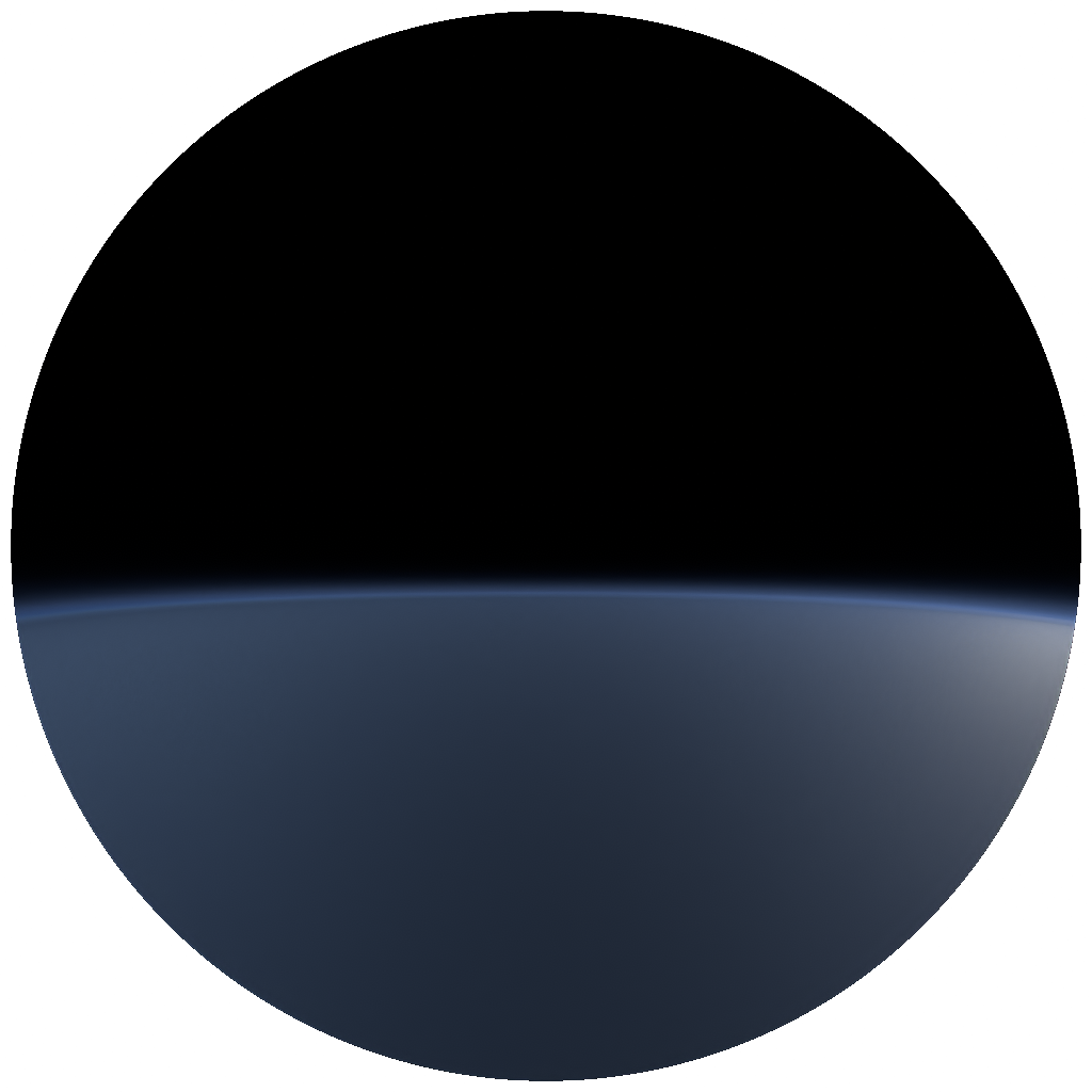
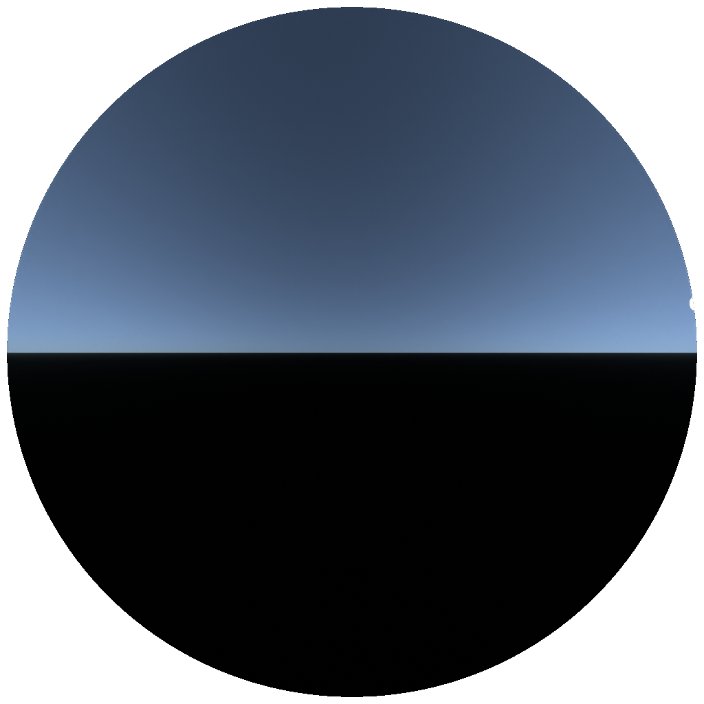
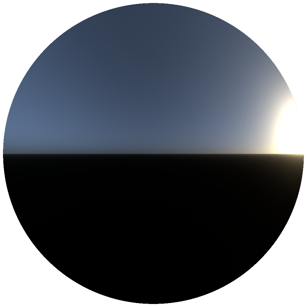
Moving the camera origin up through the atmosphere changes the sky character dramatically. At ground level the sky is a deep blue and the horizon is bright and hazy with aerosol scattering. As altitude increases the aerosol layer drops below the observer, the sky darkens toward deep indigo, and the curvature of the atmosphere becomes visible.

Alt: 0 km · 10 λ · 4 bounces · 1024 spp · 18188.2 ms	Alt: 10 km · 10 λ · 4 bounces · 1024 spp · 16332.1 ms	Alt: 45 km · 10 λ · 4 bounces · 1024 spp · 2067.63 ms	Alt: 75 km · 10 λ · 4 bounces · 1024 spp · 194.714 ms

Also from the side-view

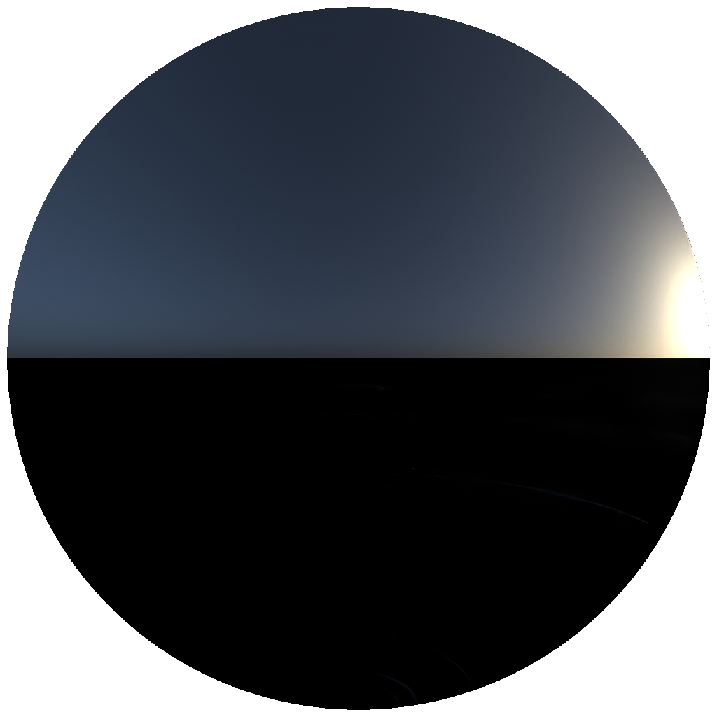Alt: 0 km · 10 λ · 4 bounces · 1024 spp · 18188.2 ms	Alt: 10 km · 10 λ · 4 bounces · 1024 spp · 16332.1 ms	Alt: 25 km · 10 λ · 4 bounces · 1024 spp · 2067.63 ms	Alt: 75 km · 10 λ · 4 bounces · 1024 spp · 194.714 ms

Aerosol Visibility

By scaling the aerosol extinction coefficients uniformly it is possible to simulate different atmospheric visibility conditions — from crisp clear days to thick haze. The continental average profile is used as the baseline (scale = 1×); the images below show progressively heavier aerosol loading.

Aerosol: 0× (Rayleigh only) · 40 λ · 4 bounces · 1024 spp · 4134.61 ms	Aerosol: 1× (baseline) · 40 λ · 4 bounces · 1024 spp · 9724.61 ms	Aerosol: 5× · 40 λ · 4 bounces · 1024 spp · 11593.1 ms	Aerosol: 10× · 40 λ · 4 bounces · 1024 spp · 12866.5 ms

With aerosols removed entirely the sky is a pure Rayleigh sky — vivid blue with no horizon haze. At 5–10× the horizon becomes a bright white-grey band and the sun disk is visibly attenuated, reproducing the look of a hazy or polluted atmosphere.

Noise and Denoising

At 1024 samples per pixel the renderer is already quite clean for the sky dome, but some residual noise is visible in regions with complex multiple-scattering paths near the horizon. The good news is that the RTX 3090 renders 1024 samples at 1K resolution in approximately nine seconds, which makes it practical to integrate an AI denoiser as a post-process step. The image on the right has been passed through a denoiser.

Raw · 40 λ · 4 bounces · 1024 spp · 9792.86 ms	Denoised · 40 λ · 4 bounces · 1024 spp · 9769.19 ms

With denoising in the pipeline, the brute-force renderer becomes a genuinely practical ground-truth tool — fast enough to produce clean reference images for a wide range of sky conditions without the hours-long render times that would otherwise make per-frame comparisons impractical.

What Works / What Doesn’t Work

What Works

The renderer produces physically accurate skies across the full range of sun elevations and viewing conditions — something a tuned RGB renderer simply cannot do. Because it works directly from measured spectral data with no fitted approximations, it isn’t bound to a minimum sun elevation, a fixed number of wavelength bins, or a pre-baked number of volumetric bounces. Everything is a runtime parameter.

The memory footprint for all atmospheric data is well under a megabyte. There are no precomputed tables to store or invalidate, and no fitted model that breaks down outside its training distribution.

The rendering speed is also a genuine surprise. At 1024 samples per pixel and 1K resolution the RTX 3090 finishes in roughly nine seconds, which paired with an AI denoiser makes this a practical ground-truth tool rather than a theoretical one.

What Doesn’t Work (Yet)

The renderer lives in its own world. It produces spectral radiance values that look correct, but porting any of this back into the main RGB-only renderer is non-trivial. A hybrid RGB–spectral system where the atmosphere is evaluated spectrally and then projected into RGB for the rest of the render is one path forward, but maintaining two rendering pipelines with different internal representations comes with real long-term costs.

The other hard limit is twilight and below-horizon sun angles. Once the sun drops below roughly −5°, the dominant sky signal comes from very long multiply-scattered paths through an optically thick horizon — paths that require a large number of bounces to converge. Below images show the undenoised raw outputs for decreasing solar angles with normalized exposure levels

Sun: −2° · 40 λ · 4 bounces · 1024 spp · 8426.8 ms	Sun: −4° · 40 λ · 4 bounces · 2048 spp · 11948.6 ms	Sun: −8° · 40 λ · 8 bounces · 16384 spp · 22745.2 ms	Sun: −10° · 40 λ · 12 bounces · 32768 spp · 28499.7 ms

Another possibility here is to utilize the technique presented in the paper Planetary Shadow-Aware Distance Sampling but this paper explicitly assumes a numerically invertible analytical atmospheric density model which was not suitable for my delta tracking system.

Next Steps

Ground albedo. The current implementation treats the planet surface as a black absorber. Wilkie et al. account for ground albedo as a spectrally varying term that bounces light back up into the atmosphere, contributing a visible brightening of the lower sky hemisphere. Adding a measured spectral albedo for common surface types (ocean, bare soil, vegetation, snow) would bring the model closer to a true physical reference and is a natural next step that the existing multiple-scattering infrastructure already supports.

Other planetary atmospheres. Earth is just one data point. The same pipeline — measured spectral composition, density profiles, and scattering coefficients fed into the same path tracer — could in principle render the atmospheres of other planets. The interesting challenge is sourcing and structuring that data: planetary atmospheric measurements come from a mix of spacecraft instruments, laboratory analogue studies, and radiative transfer models, none of which share a common format. Designing a clean data pipeline and format that can ingest this heterogeneous input and produce renderer-ready tables would make it straightforward to drop in a new planet without touching the core renderer.

Integration with the RGB renderer. The most practically useful next step is figuring out how to bring spectral accuracy back into the main renderer without a full spectral rewrite. One approach is to use the brute-force renderer as an offline oracle: render a set of sky conditions to build a compact fitted or neural representation that the RGB renderer can query at runtime. Another is a selective spectral pass — evaluate the atmosphere spectrally per pixel and convert the result to RGB only at the final accumulation step. Both approaches have trade-offs in complexity and fidelity, and comparing them against the brute-force ground truth is exactly what this renderer was built to enable.