Rendering an image is such an abstract topic, that if it’s your first encounter with render algorithms, you will most likely have a hard time understanding the concept. All the path tracing calculations, next event estimations, free flight distances and much more fancy pedantics can confuse you but, in the end, I think visualizing how a single photon moves can help you digest the concept in a better and more simplistic way.

So, in this mini-book we will be creating photon simulations inside houdini to visualize the paths of photons and see how they react to obstacles and changes in mediums (yes, we will do volume rendering. There is no avoiding that in this blog.). Then we will use this information to create ourselves a path tracer that can render many types of geometries with realistic lighting and materials.

Supporting File

This article will be consisting of 6 chapters and I’ve prepared a houdini file to accompany it while you read. If you would like to see all the vex coding and scene setups, you can purchase the file below. Every chapter is separated by object nodes and inside them you can find explanatory notes to walk you through the setups. I tried to clarify vex codes with comments and references. It is also a good starting point for the Exercises you can find at the end of each chapter.

Photon Simulation on

Chapter 1 – A Real Life Scenario

During the day we are constantly rendering objects with our eyes, cameras or sensors. It all boils down to generating a signal based on the interaction with a photon. The energy of the photon determines what we perceive as color (or heat). This is all thanks to the giant nuclear reactor that we are orbiting. Sun’s energy output is so large that it emits approximately 1 x 1045 photons per second in all wavelengths and we only receive 0.00000004534% of that. Even this amount of energy is enough to provide heat and visible light earth.

We can try to simulate this in Houdini by using particles for photons and a pop solver to advance them in space. Pop solver will give us the most important part in our photon renderer: Collision detection.

If you want a challenge you can implement a sphere or box intersection with vex but I’ve omitted that part to focus only on photons.

Besides collision detection we won’t take anything from the pop solver and we have to implement our own bounce (as an elastic collision in this case) to use as reflection, because in the next chapters we will need some photons to bounce and some to get inside the object. For a simple reflection algorithm you can check out Peter Shirley’s now famous “Ray Tracing in One Weekend“. We will use our particle’s velocity as ray direction and hit normal as the objects normal.

Now what we need is a light source that emits photons, some objects to hit, and a sensor (in this case a grid). In the example below I’ve used a sphere as a light source, three objects and a wall to simulate a room similar to Cornell box. The lighting calculation is done on “just hit” group with an absorption setup -A proportion of energy is absorbed every time photon bounces off of a surface- because in real life as photons collide with an object, they are re-emitted with the wavelength of an object’s substance and they lose the energy in other wavelengths. This energy is given to the object as heat, but we will not be computing a heat transfer (would be cool) but every time a photon hits an object, the color is subtracted from its original one using that objects color.

As photons stick to the sensor grid we start to see some basic reflections. But that is a total chaos to see thousands of photons bashing everywhere. For a better observation we can slice the scene in XZ plane and see what’s going on.

That’s better. We have started to see secondary reflections and color bleeding but the white photons with original energies are still dominating the scene. Maybe we can blast off the photons that don’t have a hit yet. What we are left is what is known as indirect reflection.

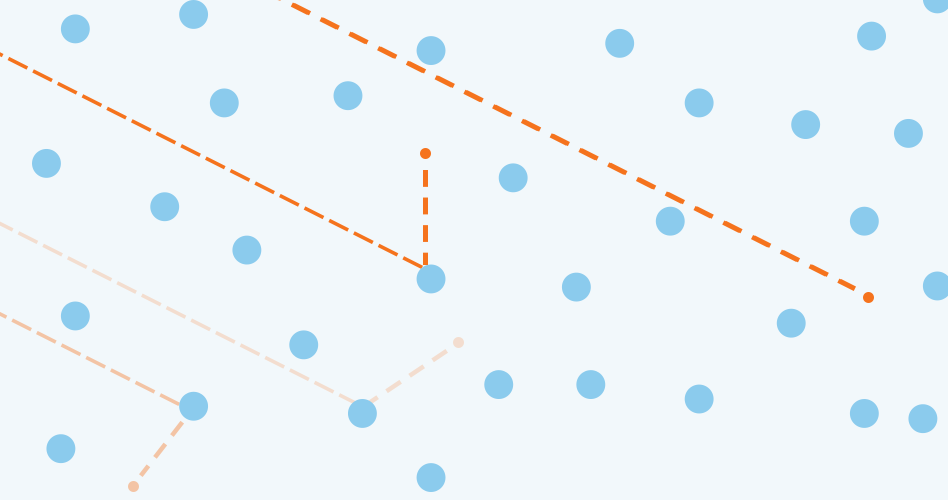
Now we can clearly see the paths of photons. The green mirror focuses the photons in a nice beam and red and blue objects start to appear on sensor. But as you will notice most of the photons just leave the room from the left side without even hitting the sensor. I’m also killing the photons with collision number larger than 5 (this will become ray depth in future chapters), so another large sum dies before even reaching the grid. So why did we even simulated those photons? We are spending a quite computational resource for such a little gain.

That is actually a problem more general than rendering. We are trying to simulate real life phenomena with limited resources. In real life there are uncountable photons traveling around at lightspeed and with our limited computing and memory power in today’s computers, It is very hard to come up with a usable solution for rendering using only rays emitted from lights.

As a solution for the very specific problem above, in the next chapter we will be emitting our photons from our camera. This way we won’t be wasting any time for a photon that might not have hit the sensor and we already know that all the photons are the ones that have a contribution to the image we want to render.

Although it may seem inefficient, don’t just throw away light photons yet. As you can see above this algorithm is very good at rendering caustics and help illuminate where camera photons can’t reach. That’s why we have algorithms like photon mapping, VCM (Vertex connection and merging – connecting light and camera rays), bidirectional rendering, etc.

Exercises

• Can you use another shape as camera sensor? How about a 3D object like a sphere, how would you map it back to 2D?
• How can you change focus point of the camera?
• How can you speed this up? How about not calculating every time step of photon? Can you forecast a collision before it happens?
• What if our light source is just a very hot object and radiates only in infrared wavelength. Can you do a heat transfer setup?
• Is heat transfer any different than light transfer?

Chapter 2 – Camera Rays

In the first chapter we tried to render an image by emitting photons from light sources and saw that it is highly inefficient. Now we will just hit the reverse button and trace a photon backwards as it starts out on our sensor, hits an object and then goes to the light source.

Doing so we will cut down our computational power usage by focusing only on the photons that ended up on our sensor. You will see that instead of calculating paths of millions of photons, simulating only a couple thousand photons are enough to start rendering.

A 640×480 image takes 307,200 photons with 1 sample per pixel. We won’t be focusing on pixels just yet but I just wanted you to know that a small size of camera rays are enough to create a scene representation.

We will also make a couple adjustments on our reflection and color calculation code. First of all we don’t have to implement our own reflection code anymore because Vex already has a reflect function which we can use with our velocity and hit normal to get the outgoing direction (you can sometimes see this as in direction because we are tracing the photon backwards in time). Secondly we have to change our color calculation from a subtractive scheme to an additive one because now that we are going back in time we are assuming that instead of losing energy, a photon gains the energy back.

So let’s remove the light source and just emit photons from the camera grid. But before doing that we will also make a change in the initial velocity of the photons. Instead of using the object normal as velocity we will place a point at the back of the grid and subtract the particle position from that points position. What we’ve just created is a simple pinhole camera.

Now this is not much different than the light photons bouncing around. Instead of losing color they just regain it back. But watch now what happens if we just import the particles back from the dop network and transfer their color back to the original camera points…

You will immediately start seeing reflections. This is the essence of ray tracing…You create rays going out of a camera and trace them back to their origin. In this scene I’ve limited the ray depth to 5 and stopped any photon that hits more than 5 times or goes out of a bounding box, But you can limit your ray depth to whatever you want and see as many reflections as you wish.

What we have just created is known as a whitted ray tracer where we recursively calculate contributions of surfaces as photons bounce off of them. This is the most simple ray-tracing you can create with a simple reflection algorithm.

In the next chapter we will take a look at a more complicated algorithm.

Exercises

• We are now unable to see the caustics that green curved surface creates in chapter 1. Why is that?
• Can we combine this with the algorithm in chapter 1?

Chapter 3 – Path Tracing

Until now we had some sorts of ray tracers. In this chapter we will be creating what is known as a path tracer. The meaning of it is that we will carry out a monte carlo integration to find out the color of the camera photon. A monte carlo integration -in simple words- is an algorithm to find the value of a function by taking random samples from it. The function we are trying to figure out in this case is the color value of a photon after it bounces multiple times in a 3D environment. Because there is no analytical solution (unless it’s a very simple scene), we have to send that photon into wild and calculate the contributions of each bounce (contribution should not imply it’s additive). And after we simulate it enough and stop it with a rejection algorithm (ray depth limit), we can say that photons color equals something.

If you would like to learn about Monte Carlo methods, I strongly suggest you go over the articles at Scratchapixel as a starting point. And not only the ones about monte carlo, you should spare a week or two to go over all articles. When you feel confident you can also check the path tracing source PBRT.

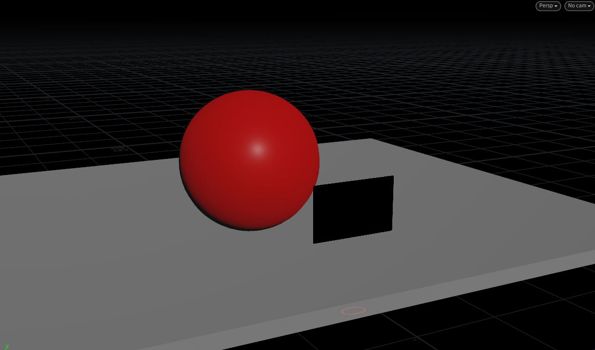
To start path-tracing we will simplify our scene a little bit to avoid the artifacts we will face with low number of samples. Since path tracers usually require large sums of samples we will place a single floor and a sphere as our scene.

And now for the changes in code, we will first change our color contribution scheme. Instead of adding or subtracting a color, we will keep an attenuation vector attribute, and as the name suggests we will attenuate this attribute every time a collision occurs. We will be updating the color as the final step in the boundary condition, that is, if a photon goes out of the scene bounds, we will stop it by putting it to sleep and update the color with a simple sky color based on velocity y direction. This idea is the implementation of CUDA version of “Ray Tracing In One Weekend” from Nvidia.

Another change will be in our collision update code. Until now we used a perfectly elastic collision to represent reflections. Now we will be implementing diffuse scattering with Vex.

Every material that we can encounter (even neutron stars) has micro elevations and dents on their surfaces. When a photon hits these surfaces they generally scatter in a direction that can be represented by a hemisphere rotated by the surface’s normal. We can implement this collision by using one of my favorite vex functions, sample_hemisphere using a vector2 comprised of two random numbers and the hit normal.

So we will now remove the reflection code from the collision updater (don’t worry we will bring it back in no time) and shoot 100,000 photons from our camera to the scene.

As photons move in space (and time), we start to see the shadows and indirect illumination for the first time. There is a nice color bleeding starting to happen in the floor near the sphere and all objects get the color of the sky. For the scene above I’ve set the ray depth limit to 50. You can see in the video below what happens if we color each ray depth by green starting from depth 0 to 30.

As you can see most of our photons just goes to sky and a very few are scattered above a depth of 10. So, a 10 ray depth might be more sensible because higher order ray depths doesn’t really contribute to the image.

Exercises

• In this scene, the color of sphere is a low value red (0.5 , 0 , 0). What happens if it had much more value, like (100.0 , 0 , 0) ?
• The bounding box is a bound node fed into a pop group node. Is making it a bounding sphere change anything?
• What is a better way for creating random numbers for the hemisphere function other then rand(@ptnum + @Frame)? Is it any important to have random numbers?

Chapter 4 – Lights

In the last chapter we have shaded our scene with a simple sky color. But in real life, sky color cannot be the only source of light. We have many types of lights such as point lights, direct (or distant) lights such as sun, lightboxes in various shapes, etc. Implementing these is not always trivial but we will do our best to represent as many shapes we can.

But, before diving into vex code and integrating various lights, there is an important architectural decision we have to take. How can we calculate the contribution of the lights? In the last chapter we added the contribution of the color as the last step when photons collided with a bounding box geometry. This is equivalent to saying “there are no more intersections that can take place” in regular ray tracing language. We can continue this approach and add the lights as collidable geometry (remember exercises 1 in chapter 3?) and add their contribution in the final step. Or we can add lights as an input to our collision update wrangle and calculate their color as a direct lighting contribution.

The first approach is called brute force path tracing, and the second one is called global illumination where we add indirect and direct illumination together. The decision we take will be affecting how we shape our algorithm so let’s take a look at both of them.

Brute Force Lighting

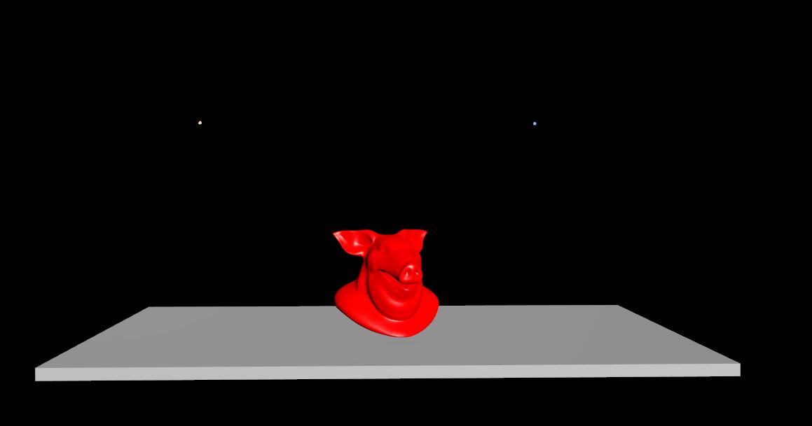
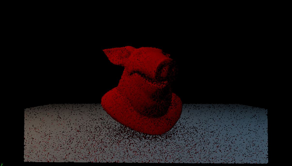
As we mentioned earlier let’s add our light geometry to our scene as hitable objects and give them a nice color to do a more realistic rendering. For the scenes below I’ve placed a sphere and a grid to represent the lights. But before doing so let’s also get rid of that sphere we put in last chapter and replace it with the staple of Houdini R&D: the test pig head.

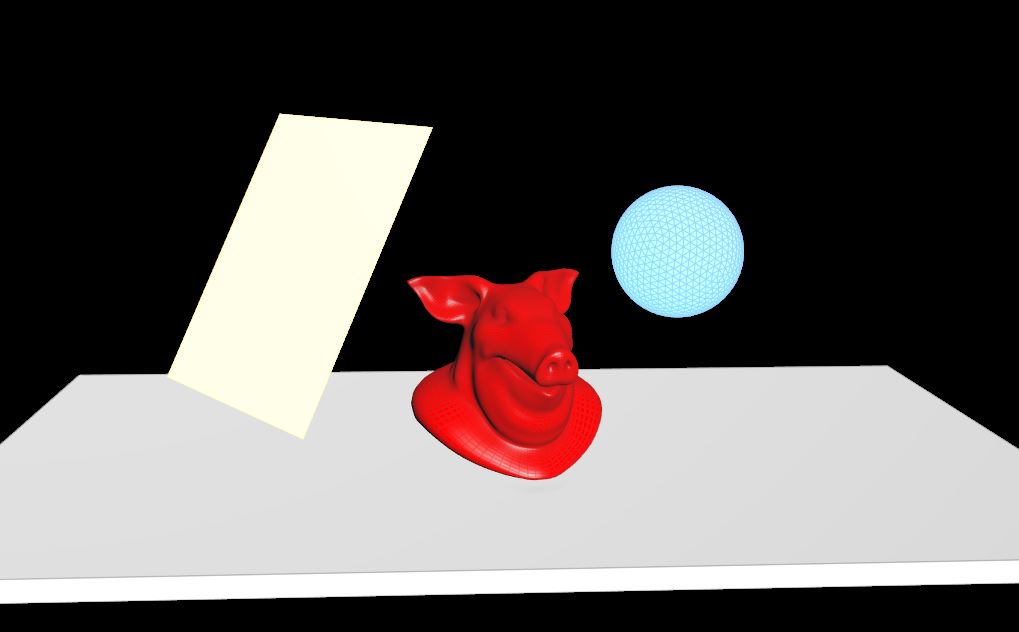
We can now shoot our photons into the scene and create another group called “light” when they hit the light geometry. We will use this group to stop the photons and send them to color calculation group. After all, this was our initial aim: Trace the photons until they reach their origin. Photons hitting the light group have found their origin and can’t go further than that.

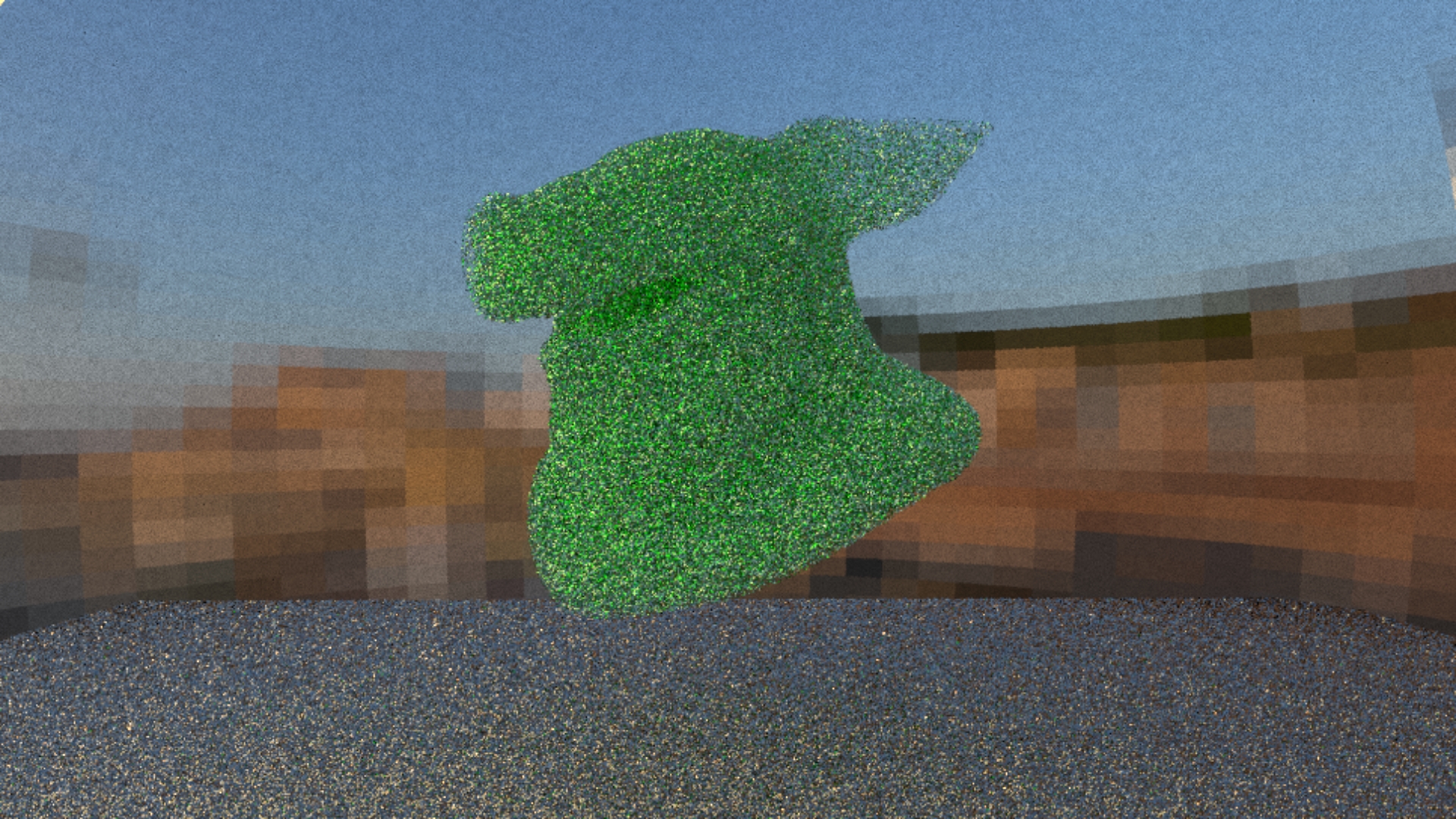
Shooting 1,000,000 photons into the scene gives us the following situation.

You can start to see nice soft shadows and light attenuation but even a million photons do not seem enough to clear the noise. This is the problem with the brute force rendering that it requires many many samples to clear out the variance. But it also has many advantages; representing different light sources such as mesh lights, area lights or sphere lights are not a problem at all, soft shadows come without an effort, It is physically correct and is much more trivial to implement. In fact we didn’t even changed much in our algorithm.

With the increase in computational power, brute force renderers are now much more production suitable and not much slower than biased renderers. There are also many advances in smart sampling algorithms and research in SIMD code that, a brute force renderer such as arnold, is now as fast as a biased renderer. After you feel that you have some experience in reading rendering related articles, you should take a look at Solidangle’s and Disney’s research papers.

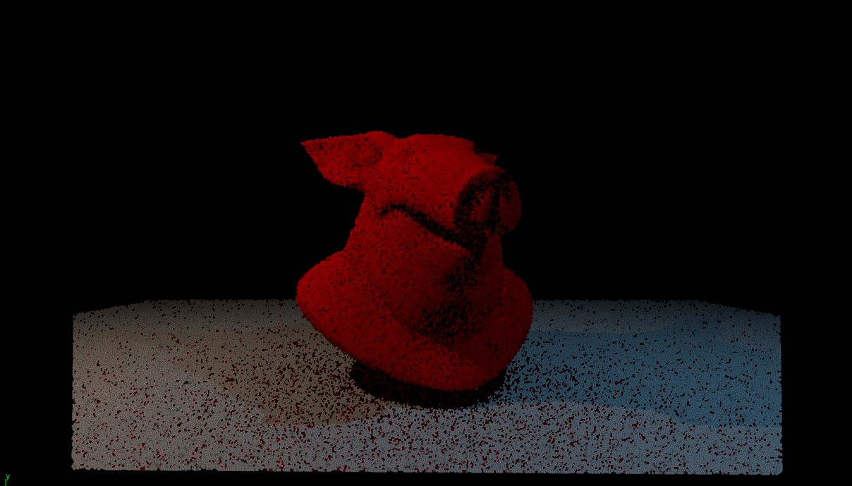
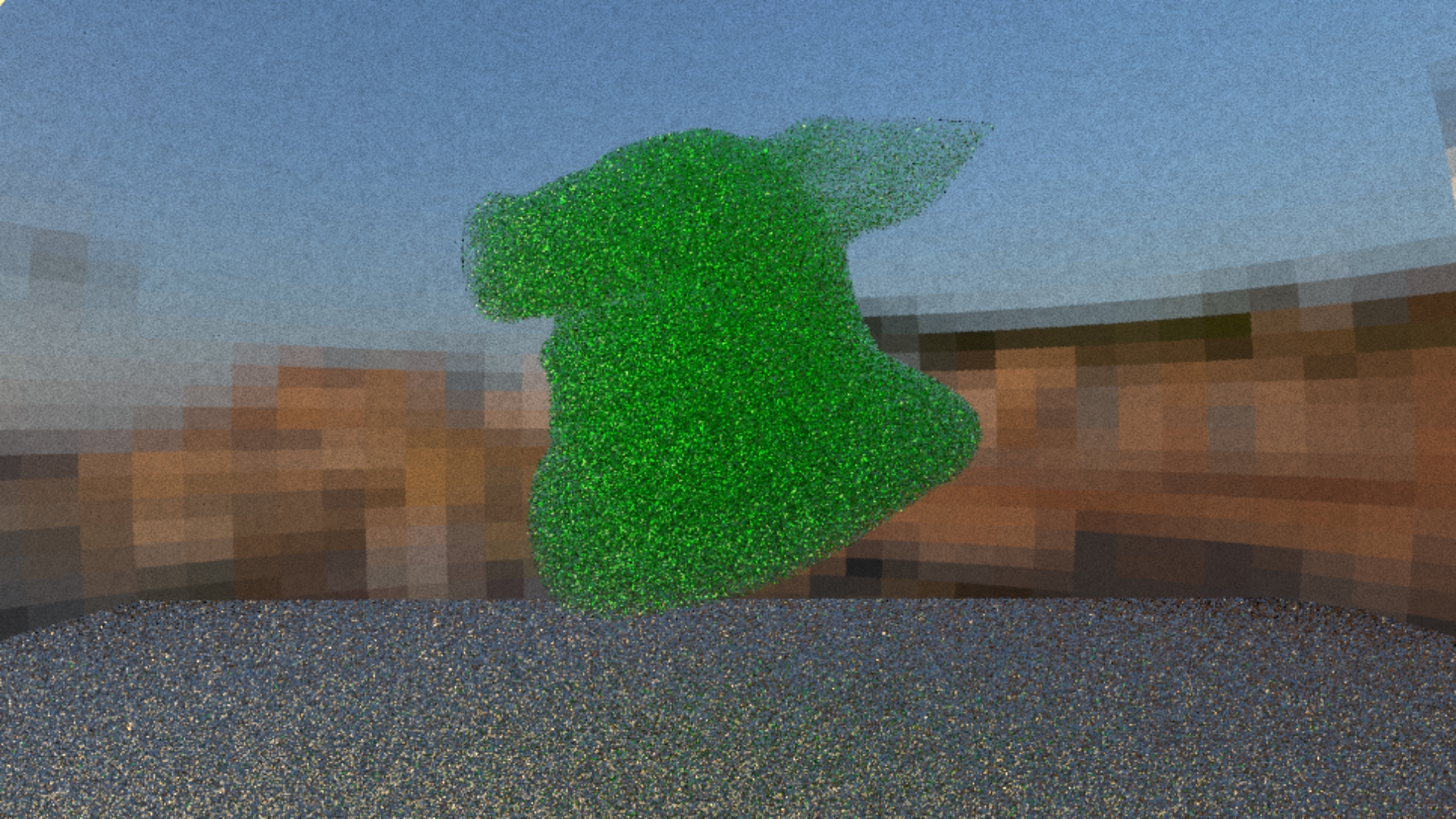
To reduce the noise however there are many techniques you can use. A better sampling scheme or simply placing more lights is one of them. But since we are doing a collision test against the light geometry it’s not wise to fill up your scene with area lights right now. Instead we can texture a simple sphere with an hdri texture and place it so it covers our whole scene.

Note: you can do this without a sphere, just convert your final velocity direction to a uv [0,1] with cartesian to polar conversion.

With an hdri image our render is now much more clean.

Direct and Indirect Lighting

Now we will take a look at how we can compute the effect of the lights by a direct+indirect lighting approach. The first thing we will change is to represent our lights with points because calculating mesh lights is not trivial as brute force rendering.

Then we will make some changes in our initial scattered points with a direct vector attribute to hold the contribution of the lights. Then in our hit wrangle using this points we will add their color to this attribute and send it to final color calculation. This will give us the following render.

Adding the color of the point lights now acts as if there was an ambient light coming from all directions equally. But according to Lambert’s cosine law the radiance a point receives from a light source decreases as the angle between the surface normal and light vector increases. We will add this by using a dot product between the hit normal and light vector.

Now we are getting a more plausible render but our point lights are missing the light decay we normally see. We can implement this by using the inverse square law with the distance from our point to the light.

We have one thing left missing and it is one of the most important steps: The Shadows.

In general rendering shadows are implemented using a shadow ray where you test against the scene geometry to see whether you can see the light source or not. But how can we achieve this ray in a particle simulation? We don’t have the luxury to send another photon towards the light direction since it would mean our photon number reaching to millions of particles in a matter of seconds. And our photons would be advancing in space-time as that shadow photon trying to reach the light point. That would be an impossible situation to manage!

As a solution this is the first time we will have to get into the world of abstraction. To see if we can see the light source from our current position we will use the houdini’s intersect function. Testing against our pig and floor box gives us a good intersection routine to multiply our light contribution.

Of course the cg environment can not be represented with point lights so we have to implement other types of lights too. But unfortunately they won’t be as trivial as brute force rendering.

Distant Light

Distant lights, or direct lights are one of the most used light in cg. They represent the light coming from a single direction. It won’t be much more different than point lights so I’ve decided that you should give it a try. Please see exercise 2 at the end of this chapter.

Area Light

Area lights are my favourite lights when doing an indoor rendering. They give soft shadows and usually a comforting look to the objects as opposed to hard shadows we see in point light etc. So let’s remove the points we have placed as lights and replace them with two rectangular grids as area lights.

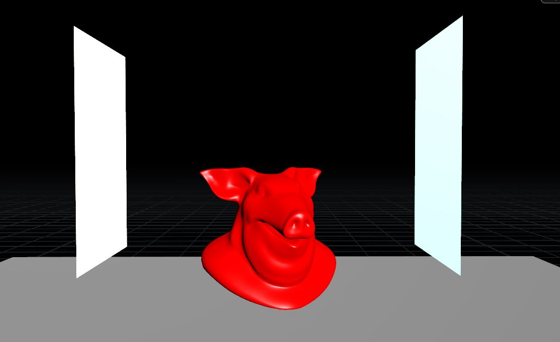
To represent an area light however we need to understand the concept of sampling. Instead of sampling a single point as we did in point lights, we will be using a sampling scheme to select a random point on the surface of the grid. For this purpose we will use the primuv function provided to us by houdini. By creating a vector uvw with random numbers in range of 0 to 1 we can choose a position corresponding to a point on grid.

Of course a single point is not enough to represent the area light, so we will encapsulate all the lighting calculations we did in the point lights in a for loop and add the contribution of each point. Finally we can divide the total light contribution with the number of samples we have taken and reach the illumination provided by that light.

You can also create a for loop to find contribution of multiple lights. Remember that this has a direct impact on render time. 2 area lights with 16 light samples gives us the beautiful soft shadows you can see below.

Note: In the next chapters we will fall back to brute force lighting because with a direct+indirect lighting approach we are assuming that our photon is somehow merged with another light photon and averaged themselves. This was not the intuition that we have started this book, We want to see how a photon behaves after it leaves the light source (or until it reaches one).

Exercises

• In brute force lighting, remove every light but the sphere light. Now make the sphere a very small radius (like 0.1 or so). How noisy is your image? Now do a * Search for “Veach MIS” on google.
• Implement a direct light. Is attenuation an option?
• How can we decrease the noise for area lights? Is taking random points on the surface a good approach?
• Our area light now gives light to both directions. Can you make it light only objects in one direction?
• How about an image? Can you make our area lights emit a texture?

Chapter 5 – Refractions

In chapter 3 we have removed our reflection code and replaced it with a diffuse scattering algorithm. In this chapter we will not only bring it back but we will also add a refraction scheme to create transparent objects like glass or water.

Before starting to implement the refraction we should do some research on the topic. We know that reflection is a simple bounce of the photon off of the surface and refraction direction is dictated by the snell’s law (Please read Scratchapixel article on shading for further info). But the refraction probability decreases as the attack angle of the photon decreases. That’s why a lake becomes a mirror like surface in the far. This ratio of refraction to reflection can be calculated by fresnel equations. And what is more complicated is that even during a refraction a phenomenon we call total internal reflection -light getting trapped inside object- can occur. You can read further into these concepts and try to implement them yourself but lucky for us Houdini has a great arsenal of functions for our use.

For the refraction to reflection ratios we will be using the fresnel function. This function does not only return the reflected/refracted ratio but is also kind enough to calculate the reflection and refraction directions, given the IOR, ray angle and surface normal.

But in the collision updater we have used a hemisphere direction for diffuse, how will we decide if a photon does a diffuse reflection, a specular reflection or goes into transmission (refraction) ?. We can do this by calculating the probabilities of a photon based on the diffuse, specular and refraction contributions. We already know that refraciton and diffuse are mutually exclusive (refraction = 1 – diffuse) but diffuse-specular and refraction-specular can live together. So we can create 3 primitive scalar attributes named refraction, diffuse and specular and calculate the probabilities as such:

@diffuse = 1 - @refraction; 
float total_prob = @refraction+@specular+@diffuse; 
f@diff_prob = fit(@diffuse,0,float total_prob,0,1); 
f@refr_prob = fit(@refraction,0,float total_prob,0,1); 
f@spec_prob = fit(@specular,0,float total_prob,0,1); 

This gives us three probabilities and we can use these in a if-else scheme in our collision updater to decide the next direction for the photon. For example if a photon hits a surface with 0.5 diffuse, 0.5 refraction and 1.0 specular it means the %25 percent of photons goes to diffuse route, %25 percent goes into material to be reflected and %50 reflects.

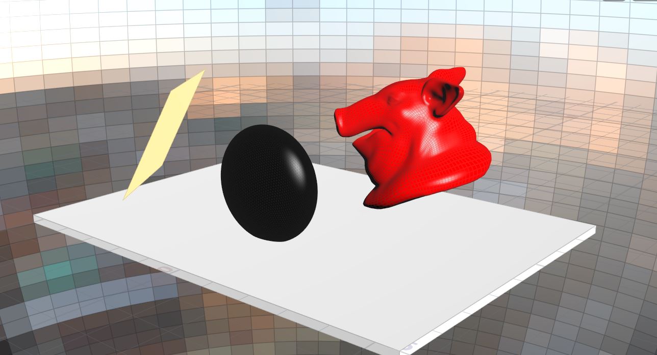
For the scene below I’ve used a totally refractive and 0.2 reflective sphere with an x radius of 0.5 , our test pighead with totally diffuse and a 0.5 specular totally diffuse floor. Tracing the photons in the scene gives us the following render.

In this very simple path-tracer we have implemented a very brute force scheme to implement refraction but you should always take a look at how other path-tracers are implemented. For an example Peter Shirley’s path tracer uses different materials with dielectric and metal shaders for path calculations. PBRT and many other path tracers use a layered system and separate each component (diffuse, refraction, subsurface scattering etc) and combine them with bsdfs. You can read a nice article on this from Wenzel Jakob at here.

Exercises

• Add specular roughness and refraction roughness. (hint: sample_direction_cone)
• Can you make glass material colored? How about color getting more saturated as the thickness of the glass increases? (hint: read next chapter and take a look at “Optical Transmission Calculator” part on this website)
• Different wavelengths refract at different ratios when transmitted through transparent objects. How can you implement this?

Chapter 6 – Volumes

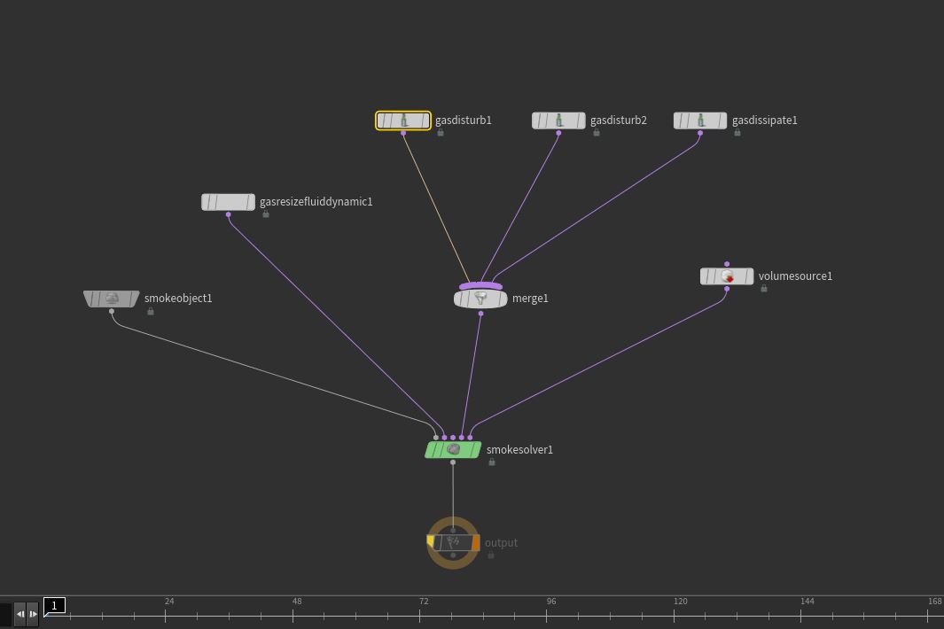
Now it’s time that you’ve been waiting all along. We will be rendering our geometry as volumes using photons.

Until now we have been advancing our photons every time step and calculating the interactions whenever there is a collision. Of course this is highly ineffective and something you wouldn’t do if you were to create a ray tracer from ground up. But it will come handy for the very first time because we will be modifying our directions and and other attributes when we are inside the volumes.

To be able to render scattering media we will make some adjustments to our algorithm. And we will need to hold a couple external (before simulation starts) attributes. For the photons we need a new attribute called “transmittance”. It is very similar to the attenuation attribute we used for diffuse and will represent the absorption due the volumes. For the render geometries however we need a couple more to represent the volumetric material. One of them is of course the density. Density will be representing the homogenous molecule density per cubic unit inside the geometry. The other ones are the volume color (or albedo), a medium toggle to tell whether the geometry is volumetric and finally an anisotropy attribute between -1 and 1 (more on that later).

Since we will be updating our photons’ attributes when they are inside the volume we will need a new group to hold the information whether a photon has entered or exited the geometry (I called this group “in_medium”). We update this group when a collision occurs and decide if photon enters or exits based on the medium attribute of primitive and the sign of dot product between velocity and surface normal.

For the volumetric calculations however we need a new wrangle to update our transmittance and photon color. Inside this wrangle we need two calculations: A rejection algorithm to stop photons based on a parameter and the transmittance calculation itself. For the rejection I’ve chosen a limit based on transmittance but a ray depth can also be implemented. In transmittance calculation we will depend on the Beer-Lambert law.

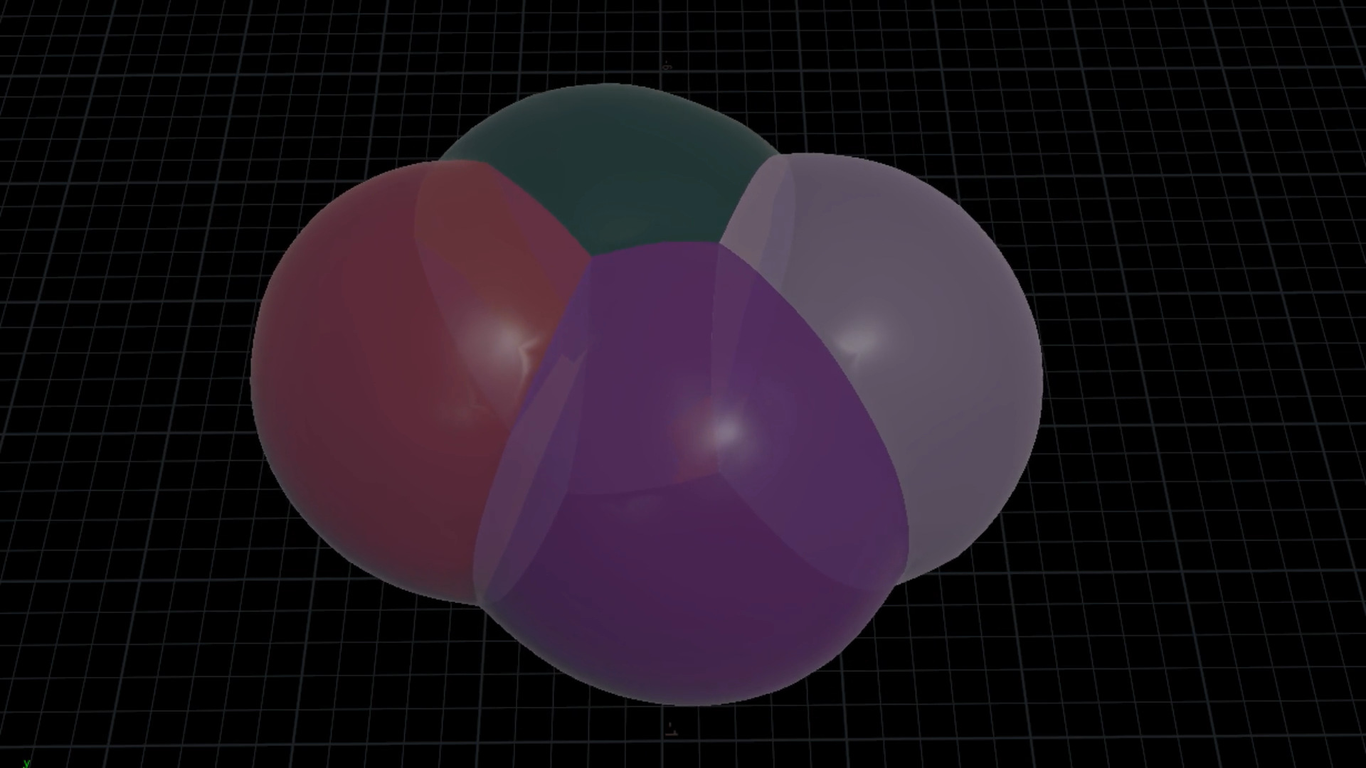
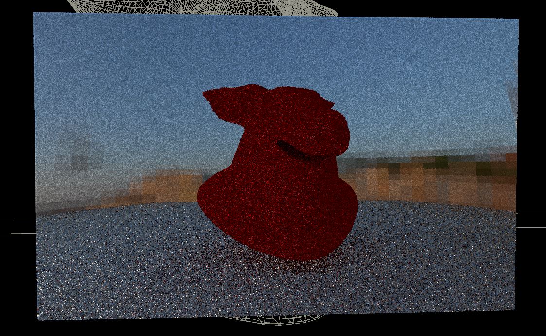
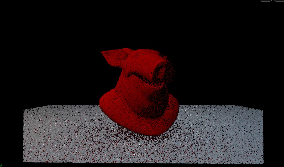
The Beer-Lambert law states that the attenuation (or absorption) correlates to the thickness of the medium and increases exponentially with the distance and an absorption coefficient. To be able to represent this we will assume that our transmittance starts with a value of 1 and decreases based on the time it spends inside the volume based on the density of it. Since we are now doing this calculation in every time step when our photon is inside the volume, finding the transmittance is trivial. For the color of the volume, we will also assume that our photon loses a wavelength based on the volume’s albedo and simply calculate it by using attenuation and volume color. You can see the final render below.

But how do we decide for the new direction of the photon?

We assume that density attribute of the volumetric primitive represents the molecule density that makes up that geometry. We can implement an algorithm where we choose to assume that a collision occurs if a random number is lower than the density and update our transmittance and color. If a collision does not happen, our photon continues it’s path. For the new direction we can -for now- assume that the direction is uniform in a sphere and the photon can take any direction.

But a uniform direction is not always the case based on the molecule composition of the volume.

Anisotropy in volumes

g parameter ranging from -0.95 to 0.95

Of course there are photons that take other directions even with a highly anisotropic parameter but what you should be caring about is the proportion of photons that take a direction.

Finally we can visualize the effect of anisotropy to our volumetric geometry. Below you can compare the effect of anisotropy parameter of -0.8 and 0.8.

Anisotropy going from 0.8 to -0.8

Exercises

• Instead of stopping photons with transmittance threshold, implement a russian-roulette rejection algorithm.
• Research a phase function other than henyey-greenstein.
• What happens if you add diffuse and specular back to volumetric geometries? Implement a system where 1/3rd proportion of photons goes into diffuse, 1/3rd goes to specular and rest goes to volumetric pathway. What did you get?
• Right now we assume that density is all uniform inside the object, How can you create a system where density is heterogenous? Can you do it with polygonal geometry? Which Vex functions do you need?

Bonus Chapter – Sandbox

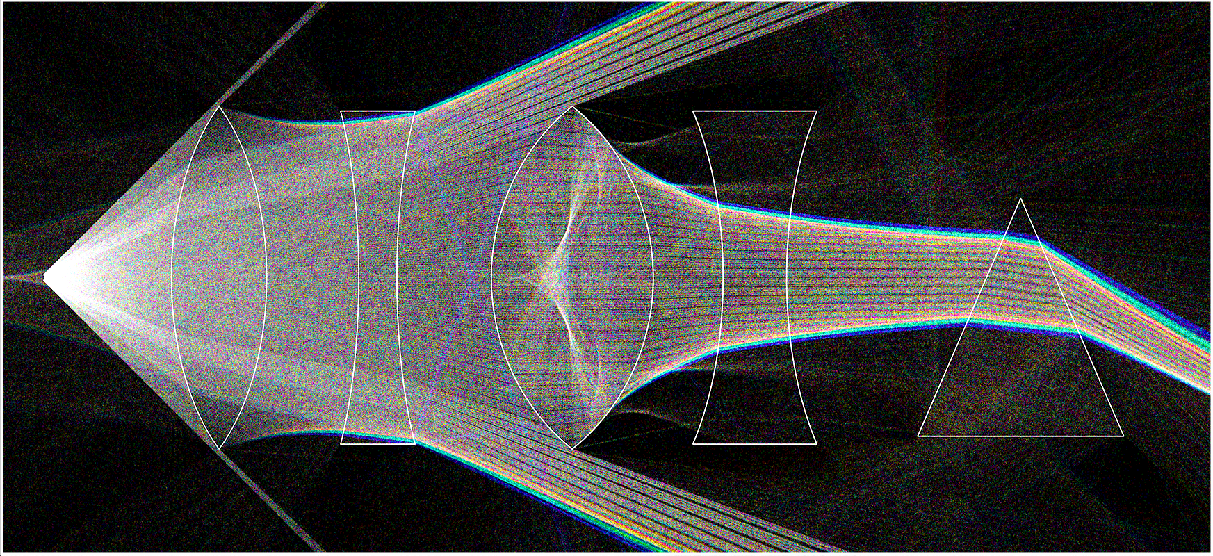
This chapter is the sandbox where you can test all your new ideas. I’ve created a 2D lens focusing setup using the refraction scheme from chapter 5 with some lenses and added color dispersion, but you are free to add whatever you want. You can bring diffuse objects, mirrors and maybe add a volume. It is always easier to see the movements of photons in a 2D setup like this.

Let your imagination run wild!

Epilogue

Congratulations, you have now completed a simple and short introduction to rendering using houdini particles. Now the whole world of rendering awaits you. If you feel like you want to read further your first stop should be Peter Shirley’s Ray Tracing in One weekend. Then you can read the articles on scratchapixel and finally look for more.

What I want to suggest to you however is that if you are interested in these topics, read PBRT as soon as possible. If you feel like it is very heavy for you, do what I did… read it like you are reading a novel. Finish the whole book in a month or so, and then implement your own renderer. Every couple months or so fall back to it and read a relevant chapter. If you want to create a physically based renderer (hobby or as a career), you eventually will have to read it anyway so it’s good to have some acquaintance.

If you are a little advanced in this topic you will most likely realise that I’ve omitted many concepts such as importance sampling, pdfs, bsdfs, etc. I wanted to keep it as simple as I can for a beginner. I consider my self only a light transport enthusiast, and I am not a professional in this field by any means. So, if you see a mistake or have a question about the exercises, you can always reach me from any medium.

Thanks for stopping by. See you on the next projects.