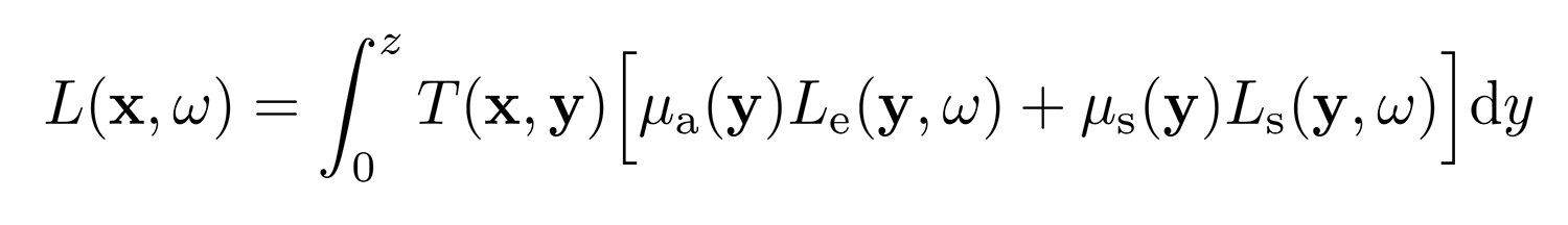Volumetric Rendering Equation (1)

Hello Again!

It’s been a long time since my last blog post, but with a good reason. I was focused on delevoping a volumetric rendering system and that almost came to an end. In these “Volumetric Path Tracing” series, I will try to share my findings and hopefully help someone who wants to start from a minimal system with actual code and explanations.

To remind you upfront that I am no expert in this field, but a mere enthusiast. I only try to convey my understanding on the topic with the purpose of helping someone out there. If you see any errors or thoughts please share, since I am also in the process of learning.

How it began?

If you know me, you know that I am obsessed with anything volumetric rendering related and you can generally catch me watching big puffy cumulus clouds.

My interest in volumetric rendering was burried for a long time, but has come to life with the release of Disney’s moana cloud data set last year. After seeing the hyperion render of that cloud, I began to inspect commercial rendering systems that could give the same result.

After a through research I found that the closest option that can give the closest look was arnold renderer. But there is a tiny problem…

Volume rendering is SLOW!!!

Rendering participating media by itself is not a complicated issue, it can even be done in real-time (real-time meaning game engine standards). But to achive the specific features of dense media (i.e. clouds), a renderer has to spend a very long time calculating the radiance coming from all directions. These calculations give the darkening at the edges and high detail in the shadowy areas. Unfortunately this means hundreds of millions of texture/material lookups and calculations.

Even though todays renderers are highly optimized pieces of engineering, we are yet to find a way other than brute force to capture true physically based unbiased rendering.

For this very reason I tried to implement my volumetric path tracer as a gpu architecture to gain leverage from the high serialization of them. And having a beginner/intermediate knowledge of CUDA helped me on the way.

My volumetric renderer is now in a stage that I am mostly happy with the results and serves me as a toy path tracer. But I want to take it further and try the new volume rendering papers and ideas from the scientific community. It features multiple scattering up to a couple of hundreds of ray bounces and reflects the features of dense cumulus clouds.

The github repo for the renderer is currently private but I am planning to make it public at the end of these series for everyone who wants to enter the world of volumetric rendering.

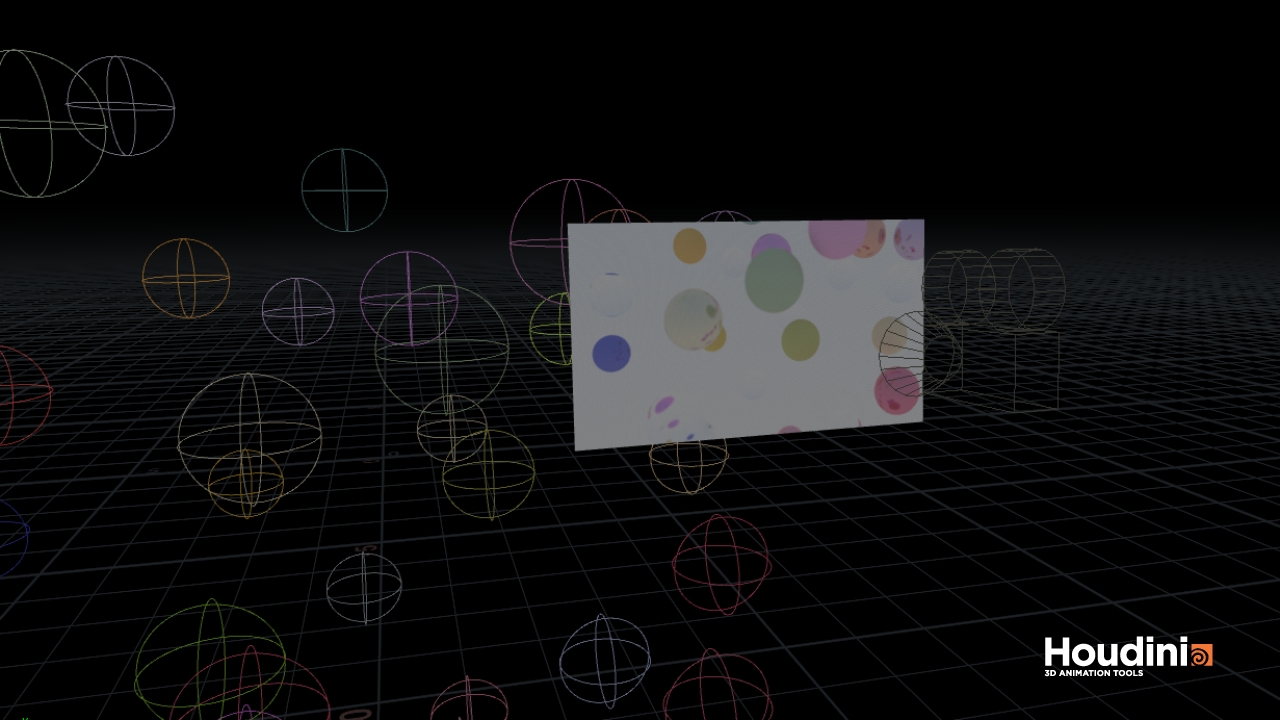
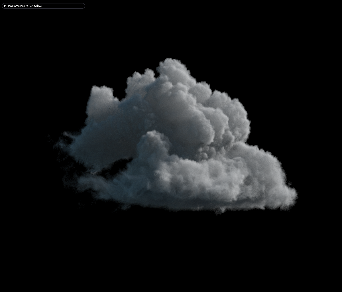
Current stage of the renderer

Lets start!

I’ve considered to start these series from the beginning and give the definitions and concepts, but eventually decided that I will leave the traditional methods and will start from the advanced topics. So instead of starting from the ground we will first build up the roof. Another reason for this, is that I feel ready to publish this one and need to find more data and research in those topics.

These building blocks will come handy in the future of series and be referred a lot. So bear with me if you are a novice and hope you find it useful if you are a professional.

What do you expect from a renderer?

Lighting artists and TD’s expect a renderer to give the most accurate results in a given time (generally a short one). And a light integrators (main part of a renderer) job is to provide lighting information based on parameters like bsdf’s and lights. We generally construct our scenes with minimal amount of lights to be able to render faster. And if it’s an outdoor scene we mostly use environment lights like HDR maps and procedurally made textures.

Procedural skys are the textures that are rendered based on a mathematical formulae and usually depend on the direction of the ray. In my path tracer I used scratchapixel’s implementation of the Nishita sky model. It uses Rayleigh and Mie model scatterings to achive color and luminosity

To find the lighting information that a point receives in a volume, an integrator sends rays towards lights and finds the radiance contribution of that light from the ray’s direction. If it’s a directional light (like sun), the direction doesn’t matter because there can be only one direction to sample. But if it’s a spherical light like our procedural sky, we need to sample based on direction.

A spherical light sampling comes with the naive solution of sending a ray in any direction inside a uniform sphere. The problem with this approach is that we don’t care about the luminosity information a texture holds and treat it like as if the volume was inside a spherical light box that recieves same value in every direction. A better approach is to send rays based on the most luminous parts of the sky. So we can achive the same quality of rendering with less rays (hence less computation time).

Spherical to uv space.

The procedural sky I’ve implemented depends on two things: ray direction and ray position. Though it’s important for larger scenes, ray position in this case doesn’t make much difference because clouds generally occupy a few kilometers in height, which is relatively small compared to few hundreds of kilometers in other directions. That’s why we will focus on ray direction.

Color in a procedural sky depends on a ray direction and we will first convert this space from a polar directions of “azimuth and elevation” to a 2D space of uv.

For this example I’ve divided the sky sphere into 180×180 image and sampled the color value in a 2π by π segments for azimuth and elevation respectively. I’ve also stored this information in a 180×180 array of floats.

Color values of sky (tonemapped)

Note: To go any further please read the pbrt section on sampling the light sources from which these ideas were implemented from

To start the sampling we need 4 textures. 2 of them are 2D textures and 2 of them are 1D textures. We will name these “marginal” and “conditional” textures.

The first texture is the conditional function texture which we will use during sampling to find the pdf (probability distribution function) that we will scale our samples with. This is important because by intentionally choosing a direction, we are messing with the true nature of spherical light direction and creating bias. Scaling by pdf gives us the true contribution from that direction. Conditional function texture is a simple length of color value and it tells us where is the highest luminosity in the space of all directions.

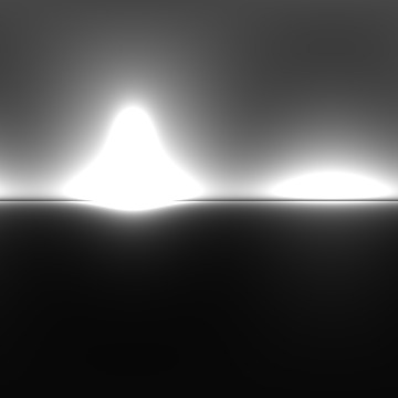Conditional function texture

As you can see the highest luminosities are in the direction of sun and below, and in the direction against it.

The second texture is the conditional CDF texture. This texture is filled by integrating each row of each column and dividing the values by the total value of that row. But before dividing each value, we will also store each total value in the 1D marginal function texture. Applying the same procedure for 1D marginal function texture we get the 1D marginal CDF texture. For brevity this textures are named after pbrt nomenclature.

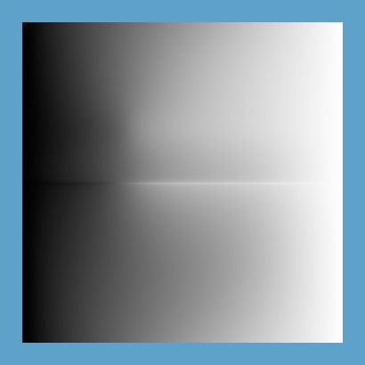Conditional CDF texture

Marginal CDF texture

note: Marginal function and cdf textures are 1D and their height is scaled for viewing purposes

How to use these textures?

The 1D marginal textures gives us the cumulative distribution and the avarage values in y-axis (avarage of rows in a column). We will use this textures to select a column first because using the 2D conditional textures alone, we wouldn’t be able to select a row before selecting a column and vice versa. Hence we use a seperate 1D texture to break this dependency cyle.

To find a column, we first choose a random number and walk the marginal cdf texture until we find the first value that satisfies that cdf(i)>xi (xi being a random number between 0 and 1). i value is the column number we want.

To see why, take a look at the marginal func and cdf textures again.

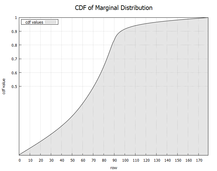
If we choose a random value of 0.9, the position to find a value that is bigger then it, is around the region in column 90. If the cdf was linear the value would be around 170. This respectively shifts our probability to choose a column in lower numbers. We can visualize this by taking a look in a violin plot that shows the densities of 4096 samples choosen based on this cdf.

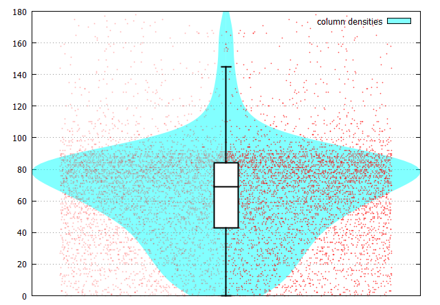Violin plot of choosen columns

You can clearly see that around 80-90 we have much more samples because the avarage density based on rows are much higher in that region.

Now that we have a column number we can go ahead and choose a row based on the 2D conditional CDF. Because this sampling depends on the 1D CDF, I hope you understand better now why they are named so.

Finding a row follows the same procedure and gives us the row number that is most likely to be choosen. After we found our column and row numbers we can visualize the points on the image.

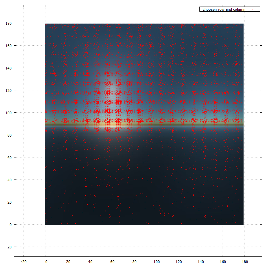uv distiribution

As you can clearly see sampling is much denser in the regions of luminous areas. And fewer at the lower hemisphere where there is not much light to sample.

Finding a ray direction from here on is straightforward. We just divide column and row numbers by height and width respectively and multiply them by π and 2π. This gives us the azimuth and elevation to convert them from a spherical coordinate to cartesian coordinate.

Calculating pdfs

As I’ve mentioned before, by choosing a direction on our own we are intentionally creating bias. To be able to achive an unbiased render we need to divide our sampled lighting information by the bias we’ve created.

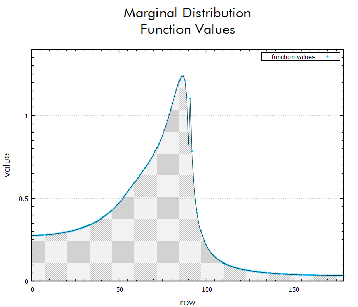
To find the pdf values we first divide the 1D marginal function value at choosen column and divide this by the total value of said texture.

Marginal pdf values (y axis scaled by 50)

Then we find the conditional pdf by value at 2D conditional function texture at choosen row and column, and divide it by 1D marginal function value at choosen row (remember these were the total values for rows). Then we simply multiply marginal and conditional pdf values.

pdf values for choosen rows and columns (y axis scaled by 50)

Finally we can visualize the directions and pdf values in a nice plot. The following 3D graph shows the directions on a unit sphere, colored according to their pdfs. Remember that the higher the pdf the lower the light contribution. We can clearly see the outline of the sun and the area below it is more dense in samples.

Choosen directions colored by pdf values

Such a sampling strategy gives us much faster sampling of the procedural sky.

Moana cloud rendered with VPT on Nvidia GTX680 with 30s of color accumulation. 5 ray depth multiple scattering, 1200×1024, 1 procedural sky and 1 sun light.

Final words.

This ends this part in our volumetric path tracing series. This is a rather advanced topic in rendering but a very crucial one. It took me a long time to figure out why pdfs were used and maybe it can even help you in topics other than rendering participating media.

In the next part I will try to briefly cover lighting and transmittance in volumetric path tracing. If you would like to get some information ahead I strongly suggest that you read “Volumetric Light Transport” in pbrt.

And I can not stress enough the importance of reading academic papers related to volume rendering if you are interested in this field. I’ve collected all the relevant volume rendering papers I could find, and uploaded them here grouped by years.

Thank you for reading. See you in the next part!

1– Monte Carlo Methods for Physically Based Volume Rendering