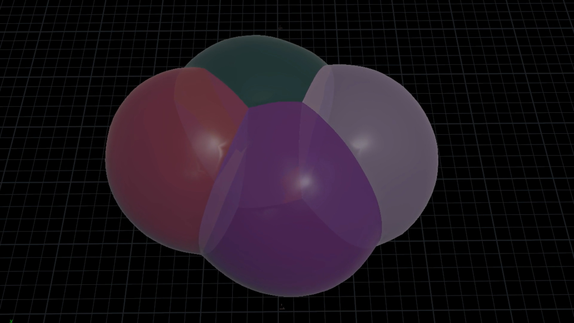
Bubbleᴴ, A Soap Film Solver
Introducing the Bubbleᴴ, A wrapper for siggraph paper "Double Bubble Sans Toil and Trouble"

Clouds are no doubt one of the main actors if you have a shot that is taking place outdoors. They can set the mood to romantic with puffy cumulus clouds, dramatic with dark, stormy clouds or epic with cumulus congestus clouds, for example if you have a dogfight scene between two fighter jets. They provide scale (especially when ground is not in shot) and help us understand the general atmosphere of the scene.
In the first two parts we have covered how to create the most common types of clouds we usually. Now that we have all the information on cloud types on various altitudes we can finally start putting them to good use. In this part we will be covering how to create the cloudscapes we see everyday. And finally we will take our chances with some exotic clouds that we may see once in a year or so.
Our main DCC software will be Houdini, for lighting and rendering we will use Arnold renderer and for compositing we will be using Davinci Fusion. For compositing we will need HDRIs and couple stock footages where necessary.
Why Arnold? Can’t I use gpu renderer for faster rendering?
Yes, you can. But with an analysis on different renderers I’ve found that Arnold is the most realistic option to use for dense clouds if you don’t have access to Disney’s Hyperion. And a long background in using arnold as a production tool in my career gave me experience in using it.
For scenes without multiple scattering you can use gpu rendering, but if you still want use another renderer for dense clouds like cumulus congestus or cumulus mediocris, mantra is still the best option -if you can afford long render times-. Terragen’s path tracer is also very good but lacks the vdb import (or instancing) features.
All the cloud setups you will see in this article are now included in the “Houdini Cloud Modelling Pack”. You can purchase them individually or as a whole pack at my gumroad page.
To start creating a cloudscape we first have to know our altitude. Since the cloud coverage depends on our visible horizon, the cloud assets we need, will be based on how far we can see. So the first thing to establish is to decide how large of an atmosphere we need. Then we will be creating our cloud assets with scales according to this.
Let’s pack our previous knowledge of cloud modelling and begin.
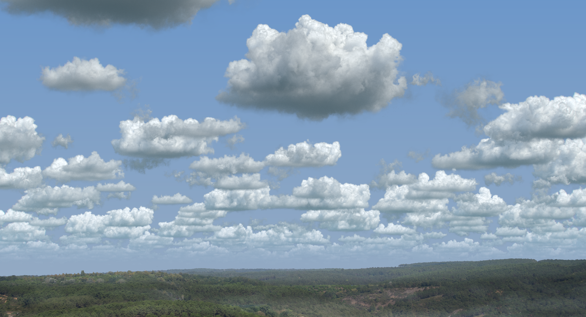
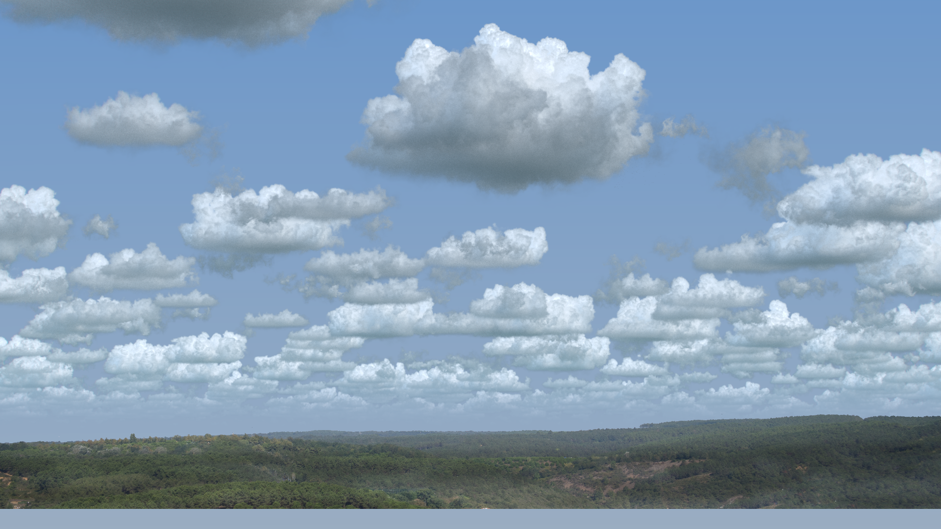
On a partly cloudy day the cloud coverage depends on the weather temperature. We will assume it’s a summer day and the location is inside a city. This means besides the atmospheric water vapour we will also need some air pollution to set our visible sky limit.
We will need a couple cumulus mediocris, and if there is slight breeze we can see some fractus clouds due convection. We will also need a slight atmospheric water vapour (and city fog) to bind them all. It is really hard to see high altitude clouds during summer days so we won’t need them right now.
We have covered creating cumulus mediocris clouds in the first part. For this scene I’ve followed the general idea to create the mediocris clouds. For the hero cloud in foreground I’ve done a simulation with 0.05 voxel division and did a composition by manually placing some fractus clouds. For the clouds in background I’ve used PDG to automate the simulation and created 15 variations with 0.1 voxel division. I’ve also created smaller darker mediocris clouds to create some variation in luminance.
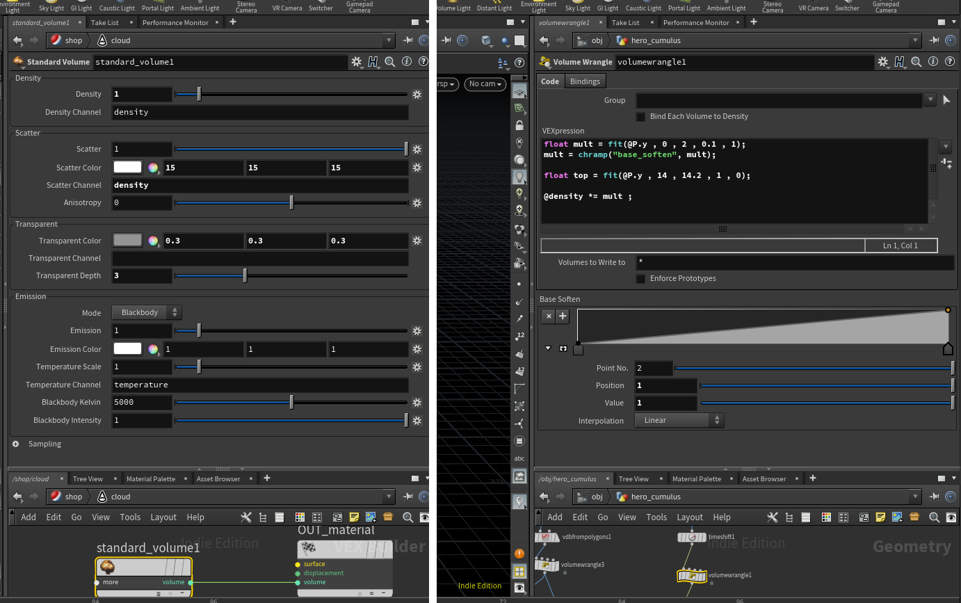
The mediocris clouds are clamped and equalized in density by using a volume wrangle to even out density all over. Then the top parts also got denser by multiplying the density with a multiplier based on voxel position.
Of course the mediocris clouds cannot live by their own. So I’ve also created 25 fractus cloud variations using PDG. The densities are multiplied by a random attribute.
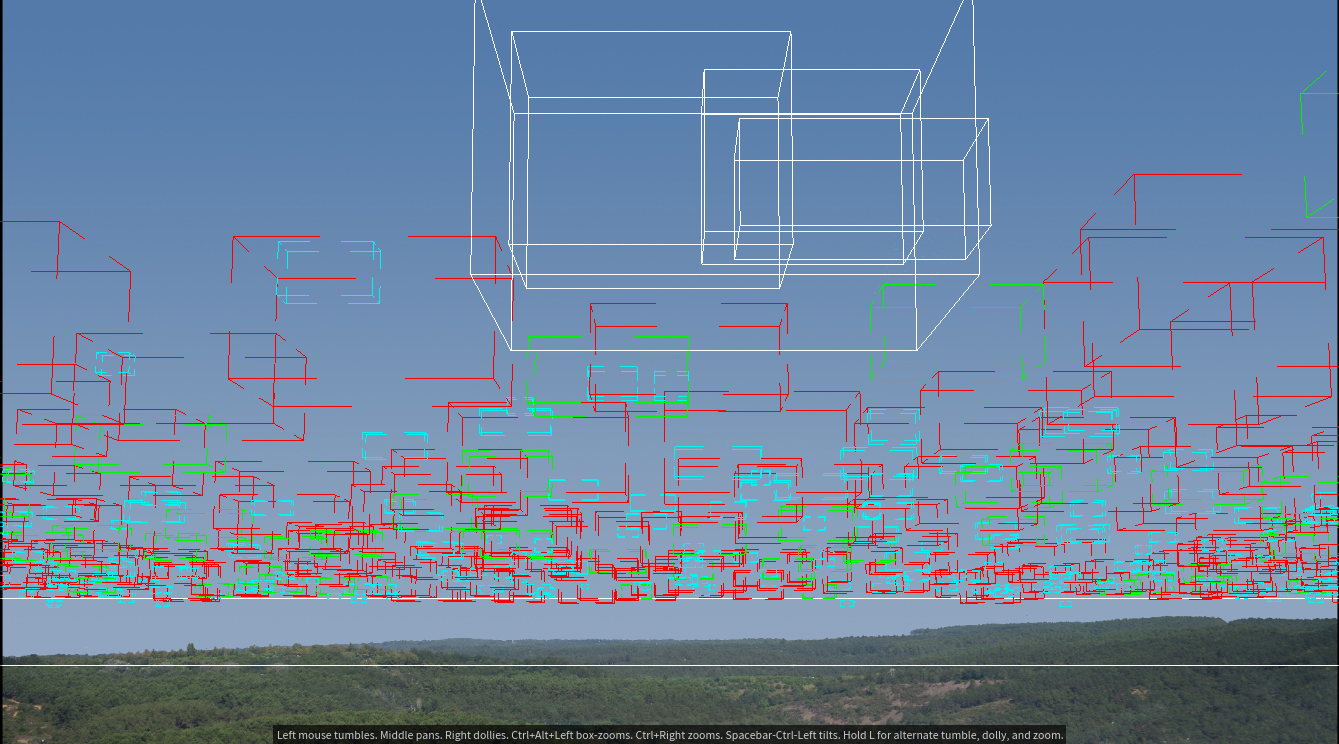
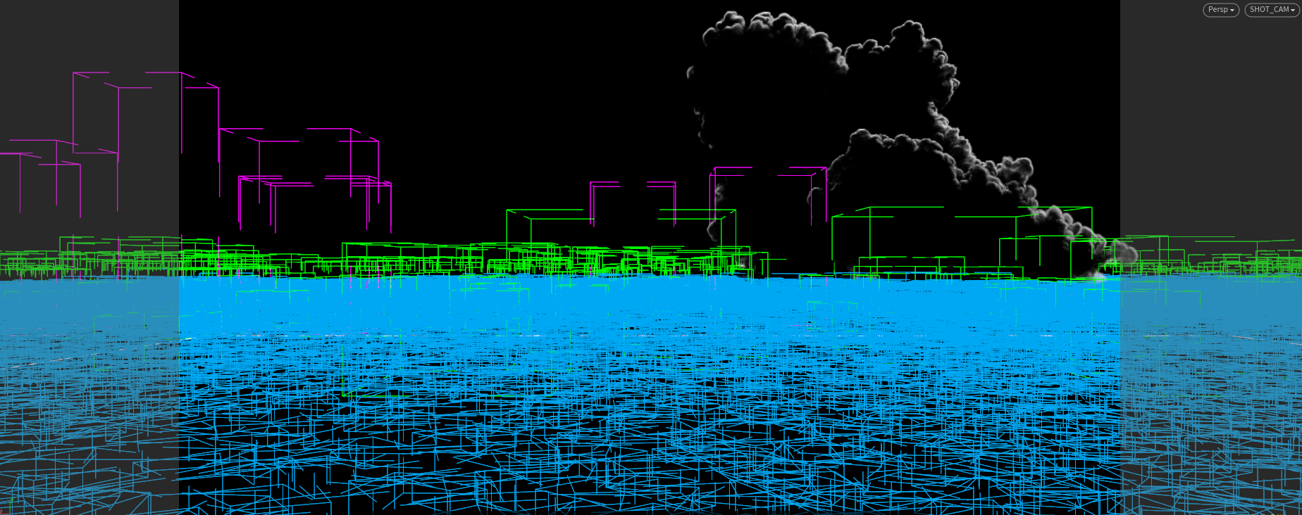
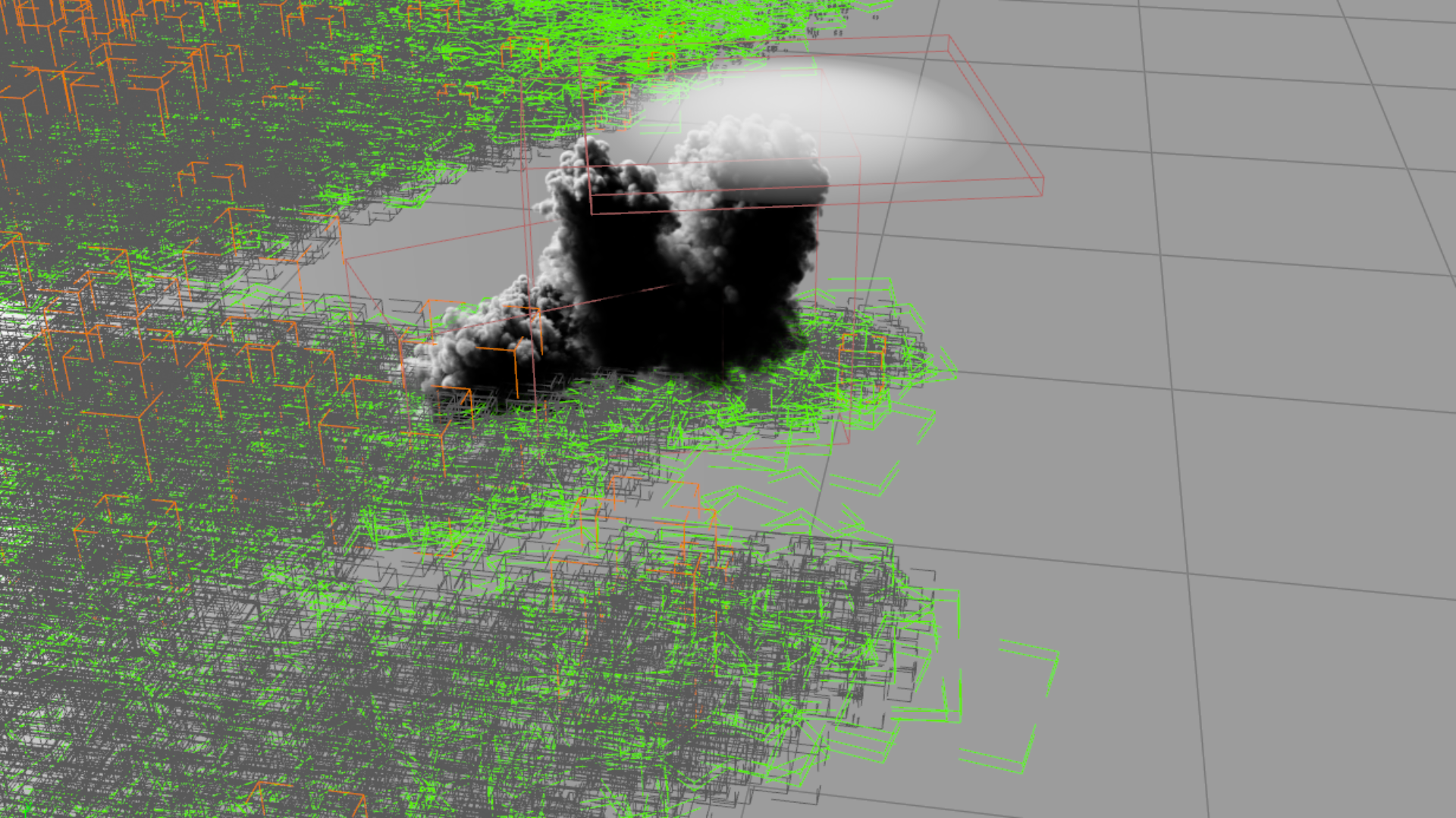
The clouds are scattered by using the instance node. First I’ve created arnold volume nodes with names of nodes pointing to vdb files. Then using the string instance attribute I’ve randomly assigned an arnold volume to a point.
The general placement is done according to the photograph I took from my balcony. The horizon was about 5 kilometers so I’ve placed the scattered points to that extent. The hero cloud is placed by hand.
For the lighting, I’ve used a skydome light with sun disabled, a distant light to simulate sunlight coming from upper right corner behind us and a distant light pointing upwards to simulate ground light and give some luminance to the bottoms of the cloud.
Shading the mediocris clouds however requires some detail. To simulate denser top parts I’ve multiplied the top of the clouds with 15. But this causes the bottom of the clouds to be very dark. In real clouds we see much more light penetration. To be able to control this I’ve copied density field into a field I’ve called transmittance and fitted the density from least dense to most dense between 1.75 to 1. This means as density get lower ray length of that part gets longer, and more light reaches the bottom of the cloud. You can see the effect below.
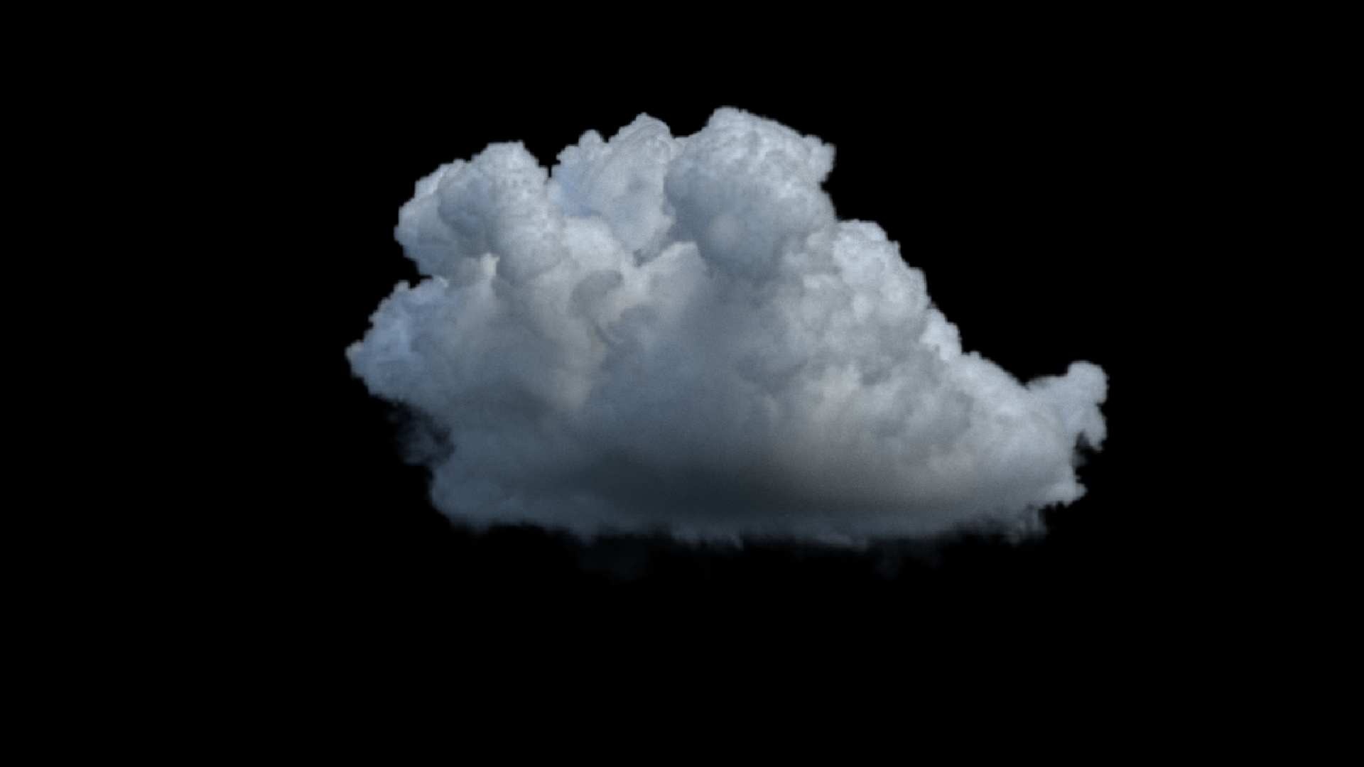
 Mapping the density max 1.75 vs 1.0
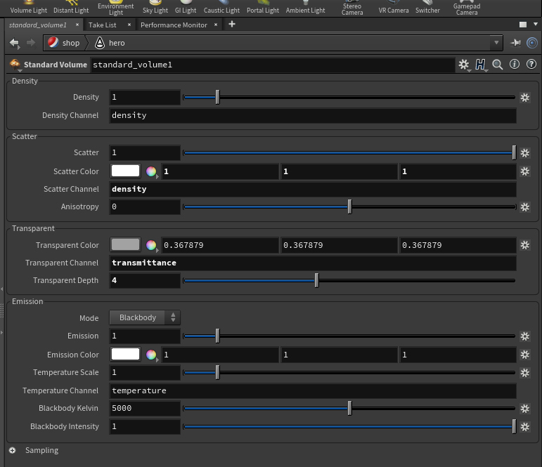
The material of the cloud is a standard volume with a little more transparent depth. Transparency depth allows you to adjust the ray length without changing density. You can see the same idea in my path tracer too.
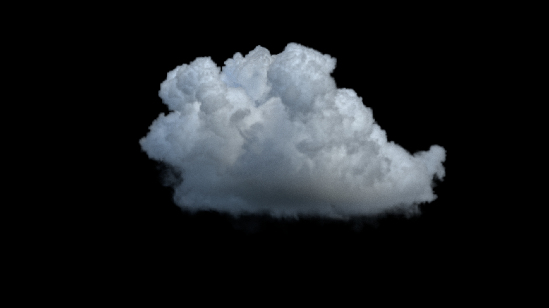
The ray depth is also a very important topic. In this image I’ve used 10 ray depth because the densest clouds we will be seeing are the cumulus mediocris clouds. And they are not as dense as cumulus congestus clouds. If I were to use one of them I would definitely go up to 100 or more. You can see the effect of the ray depth below. Please comment your opinion, which one do you like more.
 Ray Depth going from 10 to 50
Please note that comp and lighting are adjusted to ray depth. For 50 ray depth sunlight and domelight exposures are reduced. Color correction and levels are also adjusted in davinci fusion.
Going above the stratocumulus layer Commercial airplanes reach their cruising altitudes in the first 10 minutes of the flight. That means you are about 1000 meters above surface. If you have just passed the thick stratocumulus layer, it’s a perfect time to observe some cumulus mediocris and cumulus congestus clouds.
Clouds on this level depends on what you want to place in the thick layer of the strato cumulus layer. We can place a couple mediocris clouds where air convection gets higher and a couple congestus clouds on the far horizon for visual interest. We will also assume that ground is not visible at the moment and a bluish volumetric fog is also present.
We will use many of the assets we have created before but a couple new clouds are also necessary.
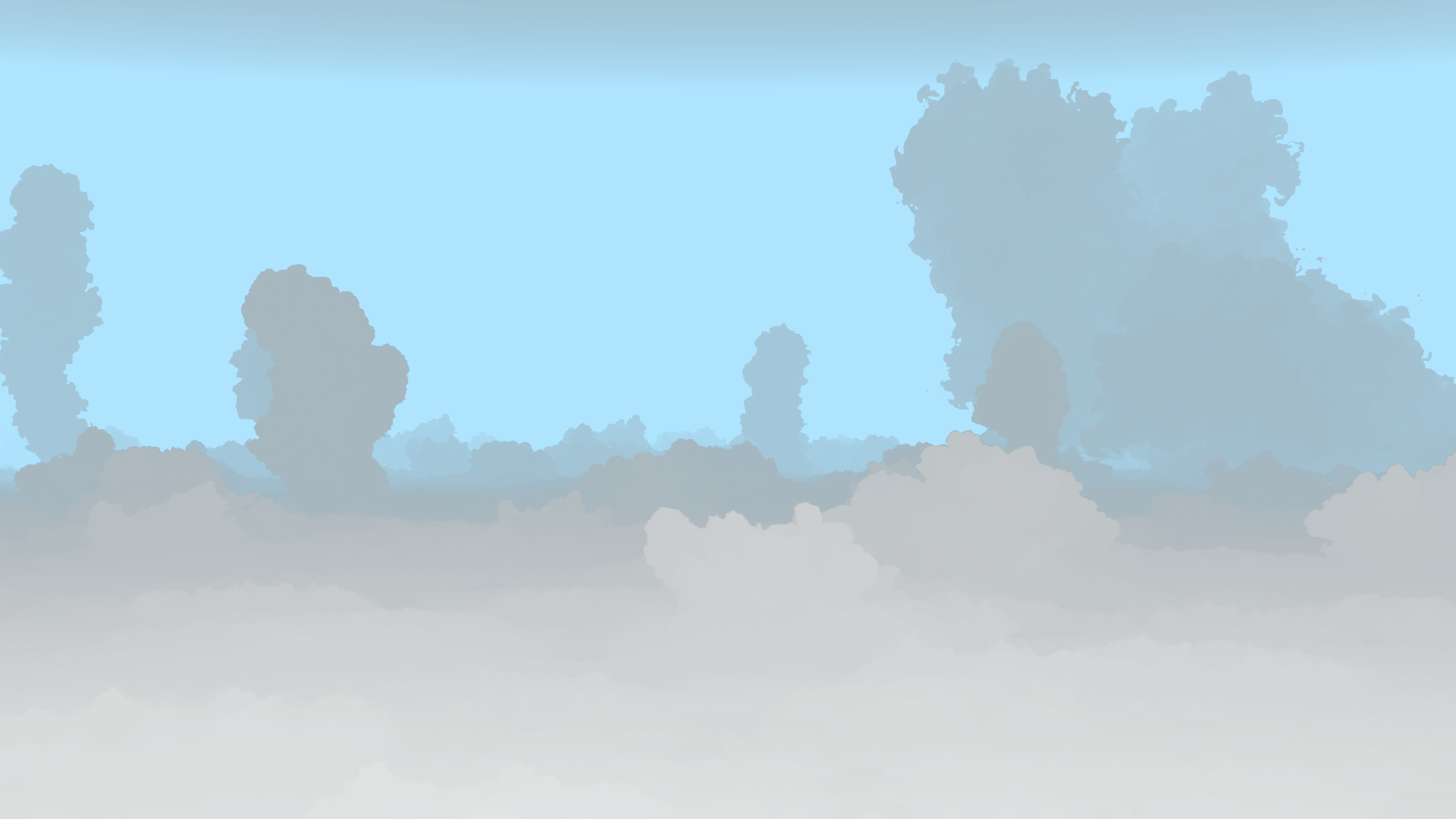
The stratocumulus is a thick layer of cumulus clouds. We will create this layer by using the ideas in mediocris cloud creation. We will start by scattering points inside a circle and adding noise to density and temperature with attribute noise node. Then we can simulate this with a low disturbance and turbulence forces to simulate the cumulus growth.
startocumulus development
If you want a lighter stratocumulus layer you can stop the simulation in an early frame. I’ve created 3 of these clouds to instance them on points. 3 variations are enough because I’ve also used rotation and pscale to create extra variation.
Towering cumulus clouds are generated by using SOP level nodes and a pyro simulation. The creation process will be explained on the next segment of high altitude view.
The clouds are again instanced using arnold volumes as instance objects. A camera frustum is used to cut the points outside of the view and a seperate mediocris layer is placed in the back to hide the lack of stratocumulus layer at the horizon level.
There are two fogs placed in the scene to simulate the fog below dew point with a greenish scattering and a high atmospheric fog above clouds with a blueish scatter.
For the lighting I’ve used a domelight with physical sky shader (sun disabled) and a distant light to simulate sunlight. Sun direction is at upper right corner coming from ~40° azimuth giving the clouds a backlit appearance.
All the shader of the clouds are standard volume with densities adjusted. For multiple scattering I’ve used 4 ray depth, because clouds are highly front scattering volumes and we are creating a backlit scene, so there is not much need for multiple scattering.
The low fog material is a standard volume with transparency distance set to 200 units to simulate a 20 km distance. The higher fog is set to 500 because it will be a thinner volumetric scattering.
Comp is done in davinci fusion. It is a very simple setup where fogs are screened over the clouds and added some glow and a lens flare.
One nice trick to use when creating cloudscapes is to create a volume depth pass. Unfortunately I couldn’t use volume depth AOV of arnold but I’ve found that using the volume albedo AOV of the higher fog (which encapsulates all clouds) and adjusting the range with a bitmap node gives a very good z-depth for volumes.
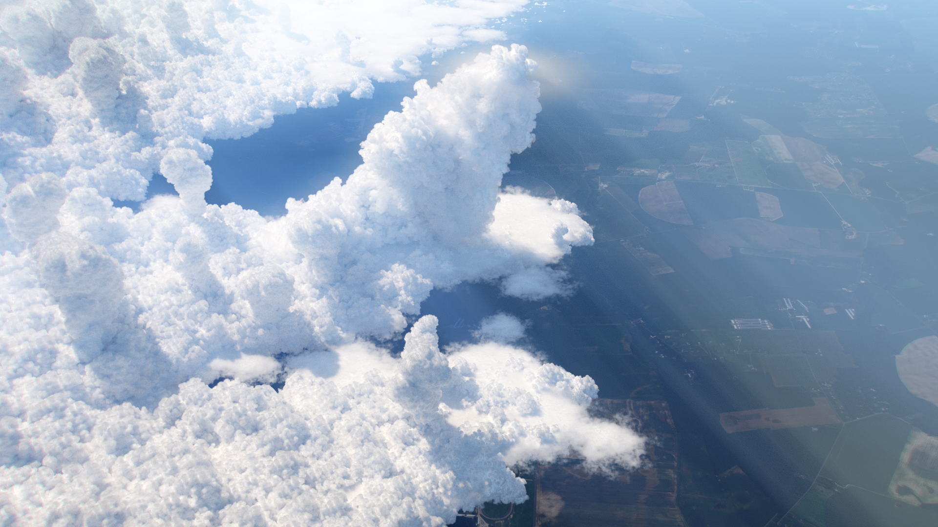
Oh, I hope they let you open the blinds because at this altitude you observe the clouds with all its glory. Your plane is typically cruising between 10 to 12 kilometers. which is above the high altitude clouds so we can see some cirrocumulus and cirrostratus clouds passing beneath us. And if the time is summer and partially cloudy down there you will have the chance to observe all the low altitude clouds.
For this scene we will need a couple of low altitude clouds; A big cumulus congestus as the hero cloud with a pileus (cap) on top of it, some cumulus mediocris clouds, a startocumulus layer to cover the base of cumulus mediocris clouds, towering cumulus clouds for added detail and two levels of fog.
The hero of our cloudscape is a collection of two clouds created with a pyro simulation that we have seen in first part of this series. They have been used together to create one big cloud. The pileus is created with basic SOP level geometry.
The base layer of the cloudscape is the cumulus mediocris and stratocumulus layer. The mediocris clouds are created with techniques we used in the first part but with a lower resolution.
The stratocumulus layer however is created with rasterizing a point collection and using “cloud noise” node. For the puffy and wispy look together I’ve used the noise mask feature of the cloud noise and created two noises, one with “abs noise” on and low roughness and one with “abs noise” off and high roughness sparse-convolution noises. This gave me a good hybrid cloud base ready to be instanced.
The towering cumulus clouds can be created by the technique we used for cumulus congestus clouds, but I’ve decided that instead of simulating hundreds of frames of simulations I could first create the base shape and run a 10 frame simulation over it.
With this in my mind I’ve created a growth system with copy-stamping a sphere based on the normal to simulate the towering mechanism. With a couple more attributes for wind and vertical height this setup gave me the base shape ready to go into a pyro simulation very similar to cumulus mediocris cloud setup.
During hot summer days you will notice a thick layer of vapour and dust beneath the dew point and a thinner bluish fog between the clouds and yourself. The vapour layer is mostly greenish-greyish due mie scattering and the upper fog layer is mostly blue due rayleigh scattering.
The two fog layers are created with simple box shapes converted into vdb fog volumes and rendered with very low density standard volume materials.
For lighting of the scene only one arnold skydome light is used. To be able to see the effects of the fog I’ve used a backlighting setup in this cloudscape with sunlight coming from upper left corner. Since we don’t see the bottom of the clouds it was unnecessary to add a ground bouncing light. All of the main clouds are rendered with 25 ray depth, fog volumes didn’t need multiple scattering.
The materials of the main clouds are standard volume with some exaggerated scattering color. I’ve used 15 as scatter color but also modified the cloud density with a volume wrangle increasing the density by height.
The general setup is divided into three parts; clouds, fog and earth. fogs are screened on cloud layer. A general bloom and flare is used for added effect. Cloud Z pass is created with using volume albedo pass of upper fog layer.
You can see the breakdown below.
Breakdown of passes used in cloudscape
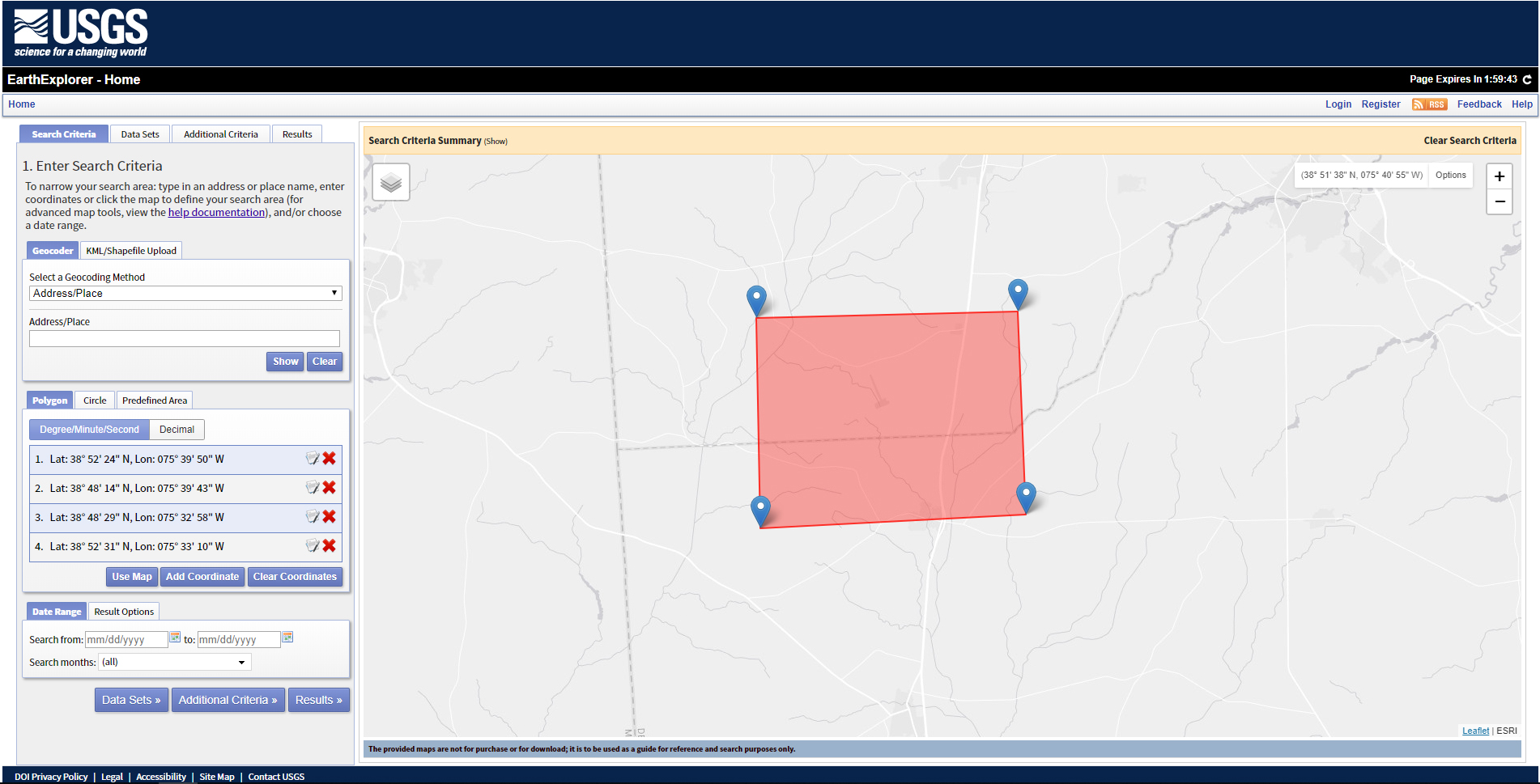
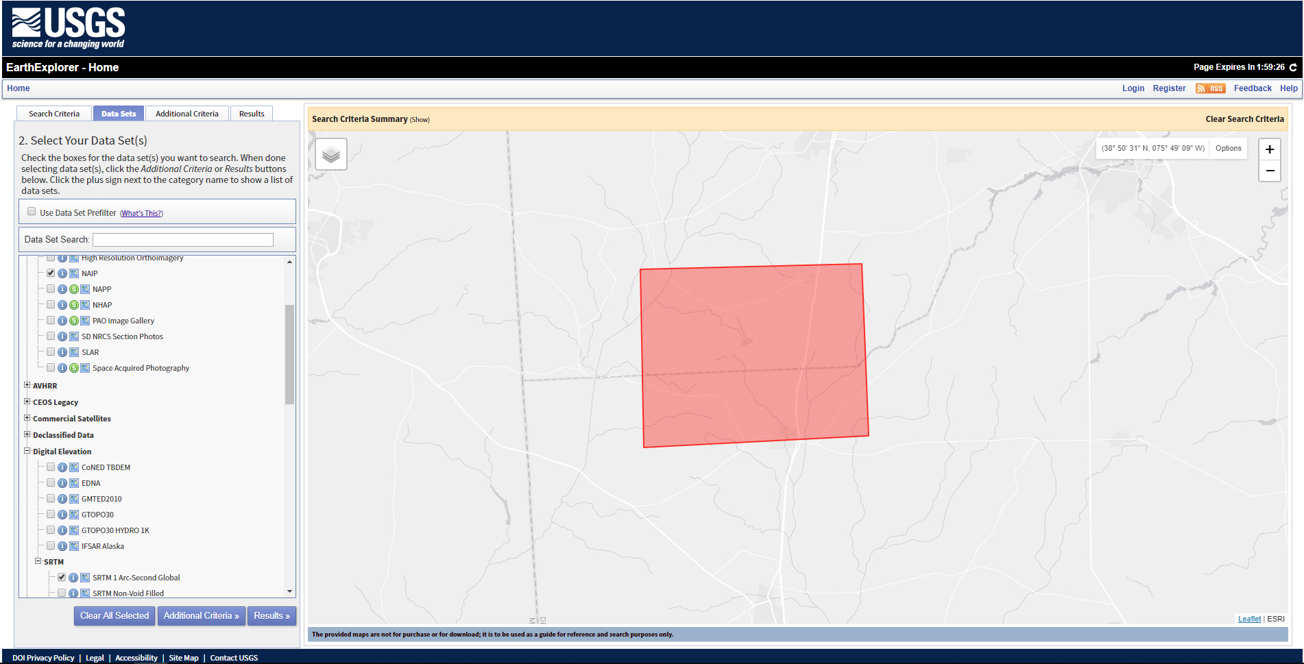
During the creation of this scene I needed very high detail textures of earth. One of the resources I found very useful is the USGS (U.S. Geological Survey) EarthExplorer website where you can find very detailed satellite images of earth. EarthExplorer is also a very good service if you need to download satellite images for a specific location.
To download the images, first visit the https://earthexplorer.usgs.gov/ and sign up for the services (you can’t download images without signing up). Now using the navigation find yourself an interesting location and select a square of your interest by clicking and selecting corner points. I’ve selected a 10×10 km region in Delaware.
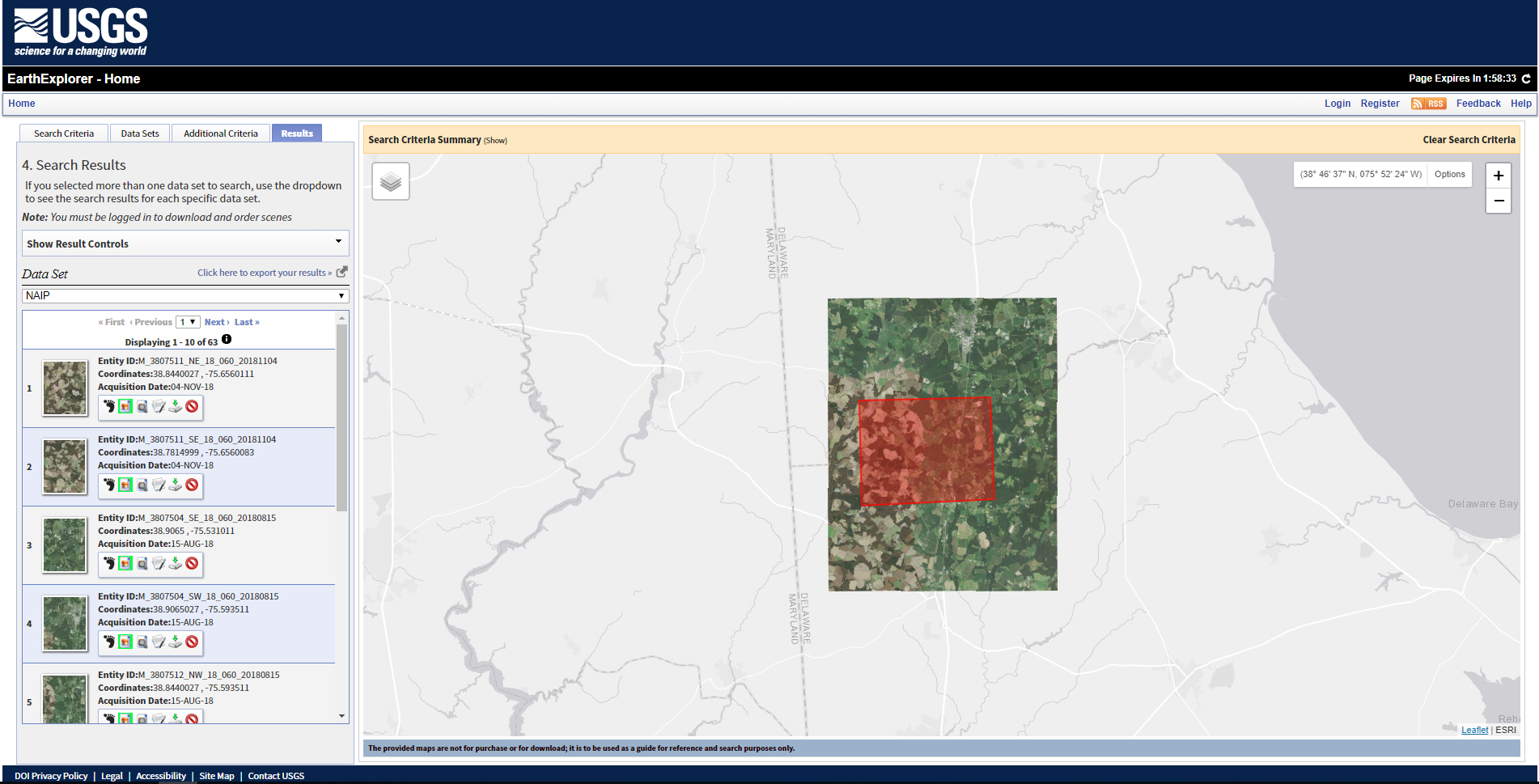
Now you have to select which datasets you want to see that includes the region you’ve just selected. I’ve found out that for diffuse textures you can select NAIP ( National Agriculture Imagery Program ) dataset under “Aerial Imagery” folder to get high detail TIFF files. You can also select “SRTM 1 Arc-second Global” under “Digital Elevation>SRTM” folder if you need height data for your ground. Entagma has a very nice tutorial on using srtm data in Houdini.
Note: srtm files can reach tens of gigabytes of data, so be prepared!
You can also explore other datasets but I’ve found that NAIP and SRTM 1 Arc-second gives the best result. After clicking the results you will be listed Dataset files that include the region you have selected. You can preview the files by clicking the image icon next to foot icon and download them as TIFF files.
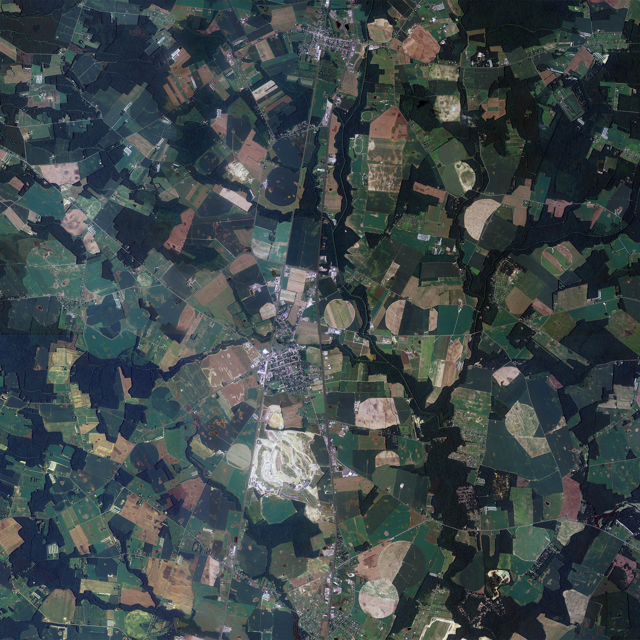
After downloading and merging the files I’ve aligned and color corrected them to my liking in photoshop. You can see the final texture below
Fluid mechanics sometimes creates very strange clouds that we may observe from time to time. I have left the creation of these clouds to the last because they are very unique and not something we see everyday. Anyway, let’s take a look at the some of the very exotic clouds.
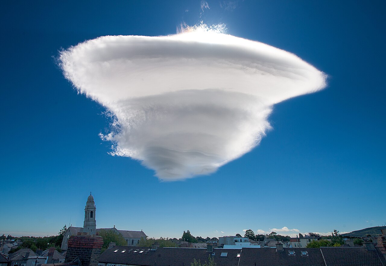 By Omnisource5 - Own work, CC BY-SA 4.0, https://commons.wikimedia.org/w/index.php?curid=41316160
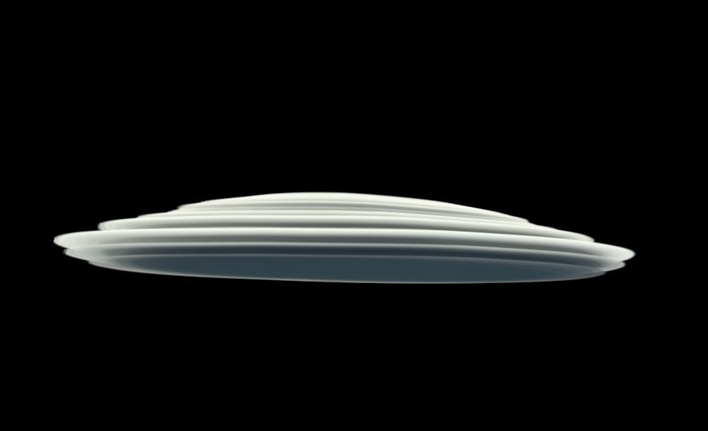
Lenticular clouds are like standing waves shaped by eddy currents (generally near mountains) in stable air. They are in fact very large condensations of water vapor climbing the mountains.
If you are a houdini person you can immediately realise that they can be simulated only with SOP level noises and a simple VDB from polygons. You can see below a VOP setup to convert a sphere to a lenticular cloud. The rest is the setup frequencies and amplitudes.
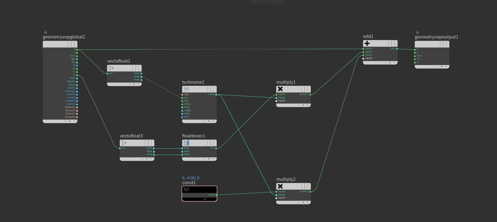
This setup gives the base shape of the cloud. You can add another level of large noise to break the shape of the cloud and even a volume wrange to add some noise to the density.
 By GRAHAMUK at the English-language Wikipedia, CC BY-SA 3.0, https://commons.wikimedia.org/w/index.php?curid=575598
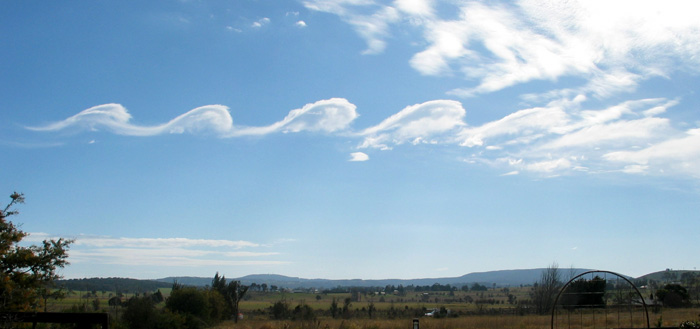
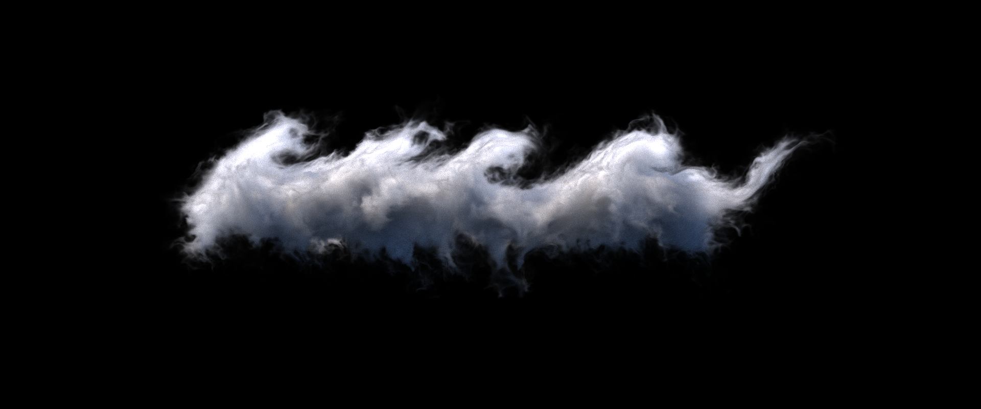
Kelvin-Helmholtz clouds form due the turbulence between two layers of fluids with different velocities. Even if they are not uncommon to see on a daily basis, seeing a large body of volume affected only by this force is quite rare.
To be able to simulate this cloud we first need some kind of Kelvin-Helmholtz instability to affect our volume. Having a volume with high velocity creates this effect but I wanted to isolate this force to modify it’s impact. To create a KH instability I’ve used entagma’s tutorial to create a 2D layer of fluid container and gave it slight gravity in -Y and -Z direction. After cutting out the part I’ve needed, I got a very good source to use as a force in smoke simulation.
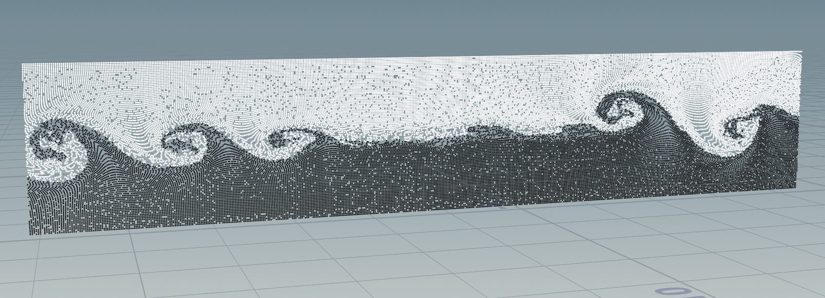
Rasterizing these points as a velocity field then I’ve feed them to a smoke simulation to create the effect I’ve needed. I’ve also added some turbulence to break the shapes.
Our cloud modelling series has came to an end with this post. I hope you enjoyed reading it as much as i enjoyed creating. The cloudscapes we see around us is of course not limited with these. I encourage you to go online and find interesting looking cloudscapes and try to create them in houdini.
The possibilities are endless when it comes to cloud modelling. Even though we haven’t covered custom shaped clouds (sculpted or modelled by a department), you can now apply these ideas to convert them to the type of cloud you want.
I hope this series help you, if you ever find yourself in need of a source to consult. Please remember that you can reach me anytime on any medium if you have anything on your mind or you see an incorrect information.
Thank you for reading and see you on the next projects.
Introducing the Bubbleᴴ, A wrapper for siggraph paper "Double Bubble Sans Toil and Trouble"
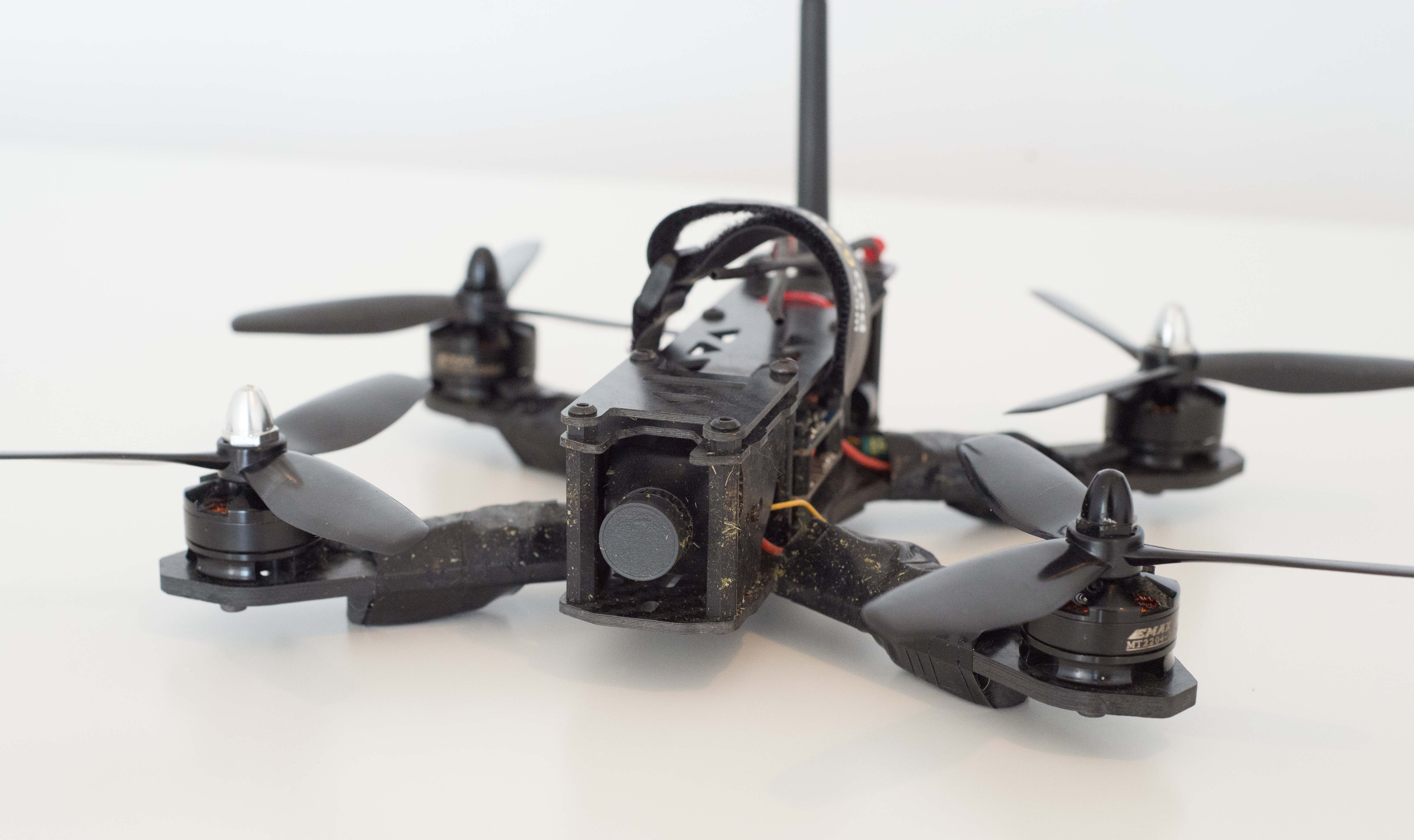
Learn how to create a path tracer using houdini particles
Learn how to create high altitude clouds with Houdini
